R E S E A R C H
Open Access
Improving palliative care with deep
learning
Anand Avati
1*, Kenneth Jung
2, Stephanie Harman
3, Lance Downing
2, Andrew Ng
1and Nigam H. Shah
2Abstract
Background: Access to palliative care is a key quality metric which most healthcare organizations strive to improve. The primary challenges to increasing palliative care access are a combination of physicians over-estimating patient prognoses, and a shortage of palliative staff in general. This, in combination with treatment inertia can result in a mismatch between patient wishes, and their actual care towards the end of life.
Methods: In this work, we address this problem, with Institutional Review Board approval, using machine learning and Electronic Health Record (EHR) data of patients. We train a Deep Neural Network model on the EHR data of patients from previous years, to predict mortality of patients within the next 3-12 month period. This prediction is used as a proxy decision for identifying patients who could benefit from palliative care.
Results: The EHR data of all admitted patients are evaluated every night by this algorithm, and the palliative care team is automatically notified of the list of patients with a positive prediction. In addition, we present a novel technique for decision interpretation, using which we provide explanations for the model’s predictions.
Conclusion: The automatic screening and notification saves the palliative care team the burden of time consuming chart reviews of all patients, and allows them to take a proactive approach in reaching out to such patients rather then relying on referrals from the treating physicians.
Keywords: Deep learning, Palliative care, Electronic health records, Interpretation
Background
The gap between the desires of patients of how they wish to spend their final days, versus how they actually spend, is well studied and documented. While approximately 80% of Americans would like to spend their final days at home if possible, only 20% do [1]. Of all the deaths that hap-pen in the United States, up to 60% of them haphap-pen in an acute care hospital while the patient was receiving aggres-sive care. Over the past decade access to palliative care resources has been on the rise in the United States. In 2008, Of all hospitals with fifty or more beds, 53% of them reported having palliative care teams; which rose to 67% in 2015 [2]. However, data from the National Palliative Care registry estimates that, despite increasing access, less than half of the 7-8% of all hospital admissions that need pal-liative care actually receive it [3]. A major contributor for this gap is the shortage of palliative care workforce [4]. Yet,
*Correspondence:[email protected]
1Department of Computer Science, Stanford University, Stanford, CA, USA
Full list of author information is available at the end of the article
technology can still play a crucial role by efficiently identi-fying patients who may benefit most from palliative care, but might otherwise slip through the cracks under current care models.
We address two aspects of this problem in our study. First, physicians tend to be overoptimistic, work under extreme time pressures, and as a result may not fail to refer patients to palliative care even when they may ben-efit [5]. This leads to patients often failing to have their wishes carried out at their end of life [6] and overuse of aggressive care. Second, the shortage of professionals in palliative care makes it expensive and time-consuming for them to proactive identify candidate patients via manual chart review of all admissions.
Another challenge is that the criteria for deciding which patients benefit from palliative care may be impossible to state explicitly and accurately. In our approach, we use deep learning to automatically screen all patients admit-ted to the hospital, and identify those who are most likely
to have palliative care needs. Since the criteria for iden-tifying palliative needs could be fuzzy and hard to define precisely, the algorithm addresses a proxy problem - to predict the probability of a given patient passing away within the next 12 months - and use that probability for making recommendations to the palliative care team. This saves the palliative care team from performing manual and cumbersome chart review of every admission, and also helps counter the potential biases of treating physi-cians by providing an objective recommendation based on the patient’s EHR. Currently existing tools to identify such patients have limitations, and they are discussed in the next section.
Related work
Accurate prognostic information is valuable to patients and caregivers (for setting expectations, planning for care and end of life), and to clinicians (for planning treat-ment) [7, 8]. Several studies have shown that clinicians generally tend to be over optimistic in their estimates of the prognoses of terminally ill patients [5, 9–11]. It has also been shown that no subset of clinicians are better at late stage prognostication than others [12,13]. However, in practice, the most common method of predictive survival remains to be the clinician’s sub-jective judgment [12]. Several solutions exist that attempt to make patient prognosis more objective and automated. Many of these solutions are models that produce a score based on the patient’s clinical and biological parameters, and can be mapped to an expected survival rate.
Prognostic tools in palliative care
The Palliative Performance Scale [14] was developed as a modification of the Karnofsky Performance Status Scale (KPS) [15] to the Palliative care setting, and is calculated based on observable factors such as: degree of ambulation, ability to do activities, ability to do self-care, food and fluid intake, and state of consciousness. The Palliative Prog-nostic Score (PPS) was constructed for the Palliative Care setting as well, focusing on terminally ill cancer patients [16]. The PPS is calculated with multiple regression anal-ysis based on the following variables: Clinical Prediction of Survival (CPS), Karnofsky Performance Status (KPS), anorexia, dyspnea, total white blood count (WBC) and lymphocyte percentage. The Palliative Prognostic Index (PPI), developed around the same time as PPS, also calcu-lates a multiple regression analysis based score using Per-formance Status, oral intake, edema, dyspnea at rest, and delirium. These scores are difficult to implement at scale since they involve face-to-face clinical assessment and involve prediction of survival by the clinician. Further-more, these scores were designed to be used within the palliative care setting, where the patient is already in an
advanced stage of the disease — as opposed to identifying them earlier.
Prognostic tools in the intensive care unit
There also are prognosis scoring models that are com-monly used in the Intensive Care Unit. The APACHE-II (Acute Physiology, Age, Chronic Health Evaluation) Score predicts hospital mortality risk for critically ill hospital-ized adults in the ICU [17]. This model has been more recently refined with the APACHE-III Score, which uses factors such as major medical and surgical disease cat-egories, acute physiologic abnormalities, age, preexisting functional limitations, major comorbidities, and treat-ment location immediately prior to ICU admission [18]. Another commonly used scoring system in the ICU is the Simplified Acute Physiological Score, or SAPS II [19], which is calculated based on the patient’s physiological and underlying disease variables. While these score are useful for the treatment team when the patient is already in the ICU, they have limited use in terms of identifying patients who are at risk of longer term mortality, while they are still capable of having a meaningful discussion of their goals and values, so that they can be set on an alternative path of care.
Prognostic tools for early identification
There have been a number of studies and tools developed that aim to identify terminally ill patients early enough for an end-of-life plan and care to be meaningful.
CriSTAL (Criteria for Screening and Triaging to Appro-priate aLternative care) was developed to identify elderly patients nearing end of life, and quantifies the risk of death in the hospital or soon after discharge [20]. CriSTAL pro-vides a check list using eighteen predictors with the goal of identifyingthe dying patient.
CARING is a tool that was developed to identify patients who could benefit from palliative care [21]. The goal was to use six simple criteria in order to identify patients who were at risk of death within 1 year. PREDICT [22] is a screening tool also based on six prognostic indi-cators, which were refined from CARING. The model was derived from 976 patients.
The Intermountain Mortality Risk score is an all-causes mortality prediction based on common laboratory tests [23]. The model provides score for 30-day, 1-year and 5-year mortality risk. It was trained on a population of 71,921 and tested on 47,458.
Meffert et al. [25] proposed a scoring method based on logistic regression on six factors to identify hospital-ized patients in need of palliative care. In this prospective study, they asked the treating physician at the time of dis-charge whether the patient had palliative care needs. The trained model was then used to identify such patients at the time of admission. The model was derived from 39,849 patients.
Ramachandran et al. [26] developed a 30-day mor-tality prediction tool for hospitalized cancer patients. Their model used eight variables that were based on information from the first 24 h of admission, and lab-oratory results and vitals. A logistic regression model was developed from these eight variables and used as a scoring function. The model was derived from 3062 patients.
Amarasingham et al. [27] built a tool to screen patients who were admitted with heart failure, and iden-tify those who are at risk of 30-day readmission or death. Their regression model uses a combination of Tabak Morality Score [28], markers of social, behav-ioral, and utilization activity that could be obtained electronically, ICD-9 CM codes specific to depression and anxiety, billing and administrative data. Though this study was not specifically focused on palliative care, the methodology of using EHR system data is relevant to our work. The model was derived from 1372 patients.
Makar et al. [29] used only Medicare claims data on older population (≥ 65 years) to predict mortality in six months. By limiting their model to use only admin-istrative data, they hypothesized an easier deployment scenario thereby making automated prognostic models more prevalent. The model was derived separately on four cohorts (one per disease type) with 20,000 patients per cohort.
Prognosis in the age of big-data
The rapid rise and proliferation of EHR systems in healthcare over the past couple of decades, combined with advances in Machine Learning techniques on high dimensional data provides a unique opportunity to make contributions in healthcare, especially in preci-sion medicine and disease prognosis [30, 31]. All the tools described above, and those we reviewed [32–36], have at least one of the following limitations. They were either derived from small data sets (limited to specific studies or cohorts), or used too few variables (intentionally to make the model portable, or avoid overfitting), or the model was too simple to capture the complexities and subtleties of human health, or was limited to certain sub-populations (based on dis-ease type, age etc.) We address these limitations in our work.
Methods
We hypothesize, as described earlier, that predicting mortality is a reasonable approximation to predicting palliative needs in patients, though palliative care is applicable more broadly beyond just end of life care, including patients still undergoing painful curative treat-ments (such as bone marrow transplants, etc). Our approach to the problem of mortality prediction is from the point of view of the palliative care team, by being largely agnostic to disease type, disease stage, sever-ity of admission (ICU vs non-ICU), age etc. The scale of data (in terms of number of patients) allows us to take a deep learning model that considers every patient in the EHR (with a sufficiently long history), with-out limiting our analysis to any specific sub-population or cohort. We frame a proxy problem statement (in place of identifying palliative needs) in a tractable way as follows:
Given a patient and a date, predict the mortality of that patient within 12 months from that date, using EHR data of that patient from the prior year.
This framing lends itself to be treated as a binary clas-sification problem, and we take a supervised learning approach using deep learning to solve it. Other than build-ing a model that performs well on the above problem, we are also separately interested in its performance on a spe-cific patient sub-population: patients who are currently admitted. This is because it is much easier for the pallia-tive care staff to intervene with admitted patients. This problem formulation and modeling has been previously described in [37].
Data source
STRIDE (Stanford Translational Research Integrated Database Environment) [38] is a clinical data warehouse supporting clinical and translational research at Stan-ford University. The data is available in the form of a relational database, from which we extract features and creating a training dataset using SQL queries. The snap-shot of STRIDE (version 6) used in our work includes the EHR data of approximately 2 million adult and pedi-atric patients cared for at either the Stanford Hospital or the Lucile Packard Children’s hospital between 1990 and 2014.
Constructing a dataset for supervised learning
In constructing a supervised learning data set, we define the following concepts:
• Positive cases: Patients who have a recorded date of death in the EHR are consideredpositive cases.
• Prediction date: The point in time, specific to each patient, that divides the patient’s health record timeline into virtual future and past events, is considered that patient’sprediction date.
Data from each patient’s virtual past is used to cal-culate the probability of their death 3-12 months in the future. Note that we must take care when defin-ing the prediction date to not violate common sense constraints (described below) that could invalidate the labels. We only include patients for whom it is pos-sible to find a prediction date that satisfies these constraints.
Positive cases
Palliative care is most beneficial when the referral occurs 3-12 months prior to death. The preparatory time required to start palliative care generally makes it too late for patients who pass away within three months. On the other hand, a lead time longer than 12 months is not desir-able either, because making accurate predictions over such a long time horizon is difficult, and more importantly, pal-liative care interventions are a limited resource that are best focused on more immediate needs. The constraints that theprediction dateshould meet for positive cases are as follows:
• Theprediction date must be a recorded date of encounter.
• Theprediction date must be at least 3 months prior to date of death (otherwise death is too near).
• Theprediction date can be at most 12 months prior to date of death (otherwise death is too far).
• Theprediction date must be at least 12 months after the date of first encounter (otherwise the patient lacks sufficient history on which to base a prediction).
• In-patient admissions are preferred over other admission types for theprediction date, as long as they meet the previous constraints (since it is easier to start the palliative care conversation with them).
• Theprediction date must be the earliest among the possible candidate dates subject to previous constraints.
Negative cases
Negative cases (patients without a date of death) are those patients who were alive for at least 12 months from the prediction date. Theirprediction dateis chosen such that it satisfies the following constraints:
• Theprediction date must be a recorded date of encounter.
• Theprediction date must be at least 12 months prior to date of last encounter (to avoid ambiguity of death after date of EHR snapshot).
• Theprediction date must be at least 12 months after the date of first encounter (otherwise insufficient history).
• In-patient admissions are preferred over other encounter types for theprediction date, as long as they meet the previous constraints (to serve as controls for the admitted positive cases).
• Theprediction date must be the latest among the possible candidate dates subject to previous constraints.
Admitted patients
These are patients whose prediction date chosen based on the above criteria happens to fall within an in-patient admission. Remaining patients (i.e, patients whose pre-diction date does not fall in range during an in-patient admission) are considered admitted. Note that non-admitted patients could still have other recorded admis-sions in their history, just theirprediction datedid not fall in one of those ranges. Further, we observe that patient records generally get updated with the latest diagnostic and physiological data, such as preliminary tests, diagnos-tics, etc. within the first twenty four hours of admission. Therefore the second day of admission is generally bet-ter suited for making a more informed prediction. Based on this rationale, foradmitted patients, we re-adjust their prediction dateby incrementing it to be the second day of admission.
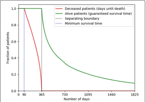
For both positive and negative cases, we censor all the data after their correspondingprediction date. The KM-plot of censor lengths is shown in Fig.1, highlighting the separation between the two classes at 365 days.
Data description
The inclusion criteria resulted in selecting a total of 221,284 patients. Table 1shows the breakdown of these patients based on inclusion and admission. Note that
Table 1Breakdown of patient counts
Alive Deceased Total
In EHR 1,880,096 131,009 2,011,105
Selected 205,571 15,713 221,284
Admitted 9648 1131 10,779
the admitted patients are kept a subset of the included patients, and not separated into a disjoint set.
We observe that, unsurprisingly, the distribution of age at prediction time is not equal between the classes, and that the positive class (of deceased patients) is skewed towards older age (Fig.2).
The included patients are randomly split in approximate ratio 8:1:1 into training, validation and test sets, as shown in Table2.
The prevalence of death among the set of all included patients is approximately 7%. Of all the included patients, approximately 5% wereadmitted patients(i.e., those who had theirprediction dateas the second day of an admis-sion). Among theadmitted patientssubset, the prevalence of death is a little higher, at about 11%.
Feature extraction
For each patient, we define theirobservation windowas the 12 months leading up to theirprediction date. Within theobservation windowof each patient, we create features using ICD9 (International Classification of Diseases 9th rev) diagnostic and billing codes, CPT (Current Proce-dural Terminology) procedure codes, RXCUI prescription codes, and encounters found in that period.
Features are created as follows. We split the observa-tion window of each paitent into fourobservation slices, specified relative to theprediction date(PD). This is done in order to capture the longitudinal nature of the data.
Fig. 2Age of patients atprediction time
Table 2Data split for modeling
Training Validation Testing
Alive 164,424 20,619 20,528 205,571
Deceased 12,587 1520 1606 15,713
177,011 22,139 22,134 221,284
The exact split points of each slice within theobservation windowis shown in Table3.
Thus,observation slice 1is the most recent, and obser-vation slice 4is the oldest. In order to give more emphasis to recent data, the slice widths are intentionally nar-row in the later slices compared to the earlier ones. Within each observation slice, we count the the num-ber of occurrences of each code in each code category (prescription, billing, etc.) in that range. The count of every such code within the slice is considered a separate feature.
We also include the patient demographics (age, gender, race and ethnicity), and the following per-patient sum-mary statistics in theobservation window for each code category:
• Count of unique codes in the category.
• Count of total number of codes in the category.
• Maximum number of codes assigned in any day.
• Minimum number of codes (non-zero) assigned in any day.
• Range of number of codes assigned in a day.
• Mean of number of codes assigned in a day.
• Variance in number of codes assigned in a day. All these features (i.e, code counts in each of the four observation slices, per category summary statistics over the observation window, and demographics) were con-catenated to form the candidate feature set. From this set, we pruned away those features which occur in 100 or fewer patients. This resulted in the final set of 13,654 fea-tures. Of the 13,654 features, each patient on average has 74 non-zero values (with a standard deviation of 62), and up to a maximum of 892 values. The overall feature matrix is approximately 99.5% sparse.
Table 3Observation window and slices
Start date End date Duration
Observation window PD - 365 PD 365
Observation slice 1 PD - 30 PD 30
Observation slice 2 PD - 90 PD - 30 60
Observation slice 3 PD - 180 PD - 90 90
Algorithm and training
Our model is a Fully Connected Deep Neural Network (DNN) [39] having an input layer (of 13,654 dimensions), 18 hidden layers (of 512 dimensions each) and a scalar out-put layer. We employ the logistic function and log loss at the output layer for binary classification (with 0/1 labels), and use the Scaled Exponential Linear Unit (SeLU) acti-vation function [40] at each layer. The model is optimized using the Adam optimizer [41], with a mini-batch size of 128 examples. The default learning rate was used (0.001).
Intermediate model snapshots of the model weights were taken every 250 mini-batch iterations, and the snap-shot that performed best on the validation test was retroactively selected as the final model. Explicit regular-ization was not found necessary. The network configu-ration was reached by extensive hyperparameter search over various network depths (ranging from 2 to 32) and activation functions (tanh,ReLUandSeLU).
The software was implemented using the Python pro-gramming language (version 2.7), PyTorch framework [42], and the scikit-learn library (version 0.17.1) [43]. The training was performed on an NVIDIA TitanX (12 GB RAM) with CUDA version 8.0.
Evaluation metric
Since the data is imbalanced (with 7% prevalence), accu-racy can be a poor evaluation metric [44]. As an extreme case, blindly predicting the majority class without even looking at the data can result in high accuracy, though as useless such a classifier may be. The ROC curve plots the trade-off between sensitivity and specificity, and the Area Under its Curve (AUROC) is generally a more robust metric compared to accuracy in imbalanced problems, but it can also be sometimes misleading [45, 46]. In use cases where the algorithm is used to surface examples of interest based on a query from a pool of data (e.g “find me patients who are near death”) and take action on them, the tradeoff between precision and recall is more meaningful than the tradeoff between sensitivity and specificity. This is generally because the action has a cost associated with it, and precision (or PPV) informs us of how likely that cost results in utility. Therefore, we use the Average Precision (AP) score, also known as Area Under Precision-Recall Curve (AUPRC) for model selection [47].
Results
In this section we report technical evaluation results obtained on the test set using the model selected based on the best AP score on the validation set.
We observe that the model is reasonably calibrated (Fig.3) with a Brier score of 0.042. In the high threshold regime, which is of interest to us, the model is a little con-servative (under-confident) in its probability estimates.
Fig. 3Reliability curve (calibration plot) of the model output probabilities on the test set data
This means, on average we expect the real precision in the selected candidates to be higher than expected.
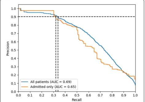
The interpolated Precision-Recall curve (with the inter-polation performed as explained in Chap 8 of [48]) is shown in Fig.4. The model achieves an AP score of 0.69 (0.65 onadmitted patients). Early recall is desirable, and therefore Recall at precision 0.9 is a metric of interest. The model achieves recall of 0.34 at 0.9 precision (0.32 on admitted patients). The Receiver Operating Charac-teristic curve is shown in Fig.5. The model achieves an AUROC of 0.93 (0.87 foradmitted patients). Both the ROC and Precision-Recall plots suggest that the model demonstrates strong early recall behavior.
Qualitative analysis
It is worth recalling that predicting mortality was only a proxy problem for the original problem of identify-ing patients who could benefit from palliative care. In
Fig. 5Receiver Operating Characteristic (ROC) of the model performance on the test set
order to evaluate our performance on the original prob-lem, we inspected false positives with high probability scores. Although such patients did not pass away within 12 months from their prediction dates, we noted that they were often diagnosed with terminal illness and/or are high utilizers of healthcare services. This can be seen in the positive and false positive examples shown in “Discussion” section.
Upon conducting a chart review of 50 randomly cho-sen patients in the top 0.9 precision bracket of the test
set, the palliative care team found all were appropriate for a referral on theirprediction date, even if they survived more than a year. This suggests that mortality prediction was a reasonable (and tractable) choice of a proxy problem to solve.
Discussion
Supervised machine learning techniques, and in partic-ular Deep Learning techniques, have recently demon-strated tremendous success in predictive ability. However, better performance often requires larger, more complex models, which comes with an inevitable cost of sacri-ficing interpretability. It is worth drawing a distinction between interpreting a model itself, versus interpreting the predictions from the model [49,50]. While interpret-ing complex models (e.g very deep neural networks) may sometimes be infeasible, it is often the case that users only want an explanation for the prediction made by the model for a given example. The utility of such an inter-pretation is generally a function of the nature of action taken based on the prediction. If the action is a high-stake action, such as an automated clinical decision, it is important to establish the trust of the practitioner in the model’s decisions for them to feel comfortable with the actions, and providing explanations along with decisions help establish that trust. In the context of our work, the action is not an automated clinical decision, but rather a tool to make the workflow of a human more efficient
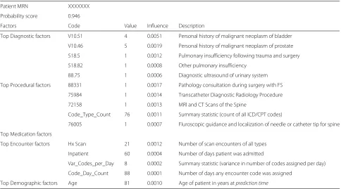
Table 4Prediction explanation generated on a random positive patient with high probability score
Patient MRN XXXXXXX
Probability score 0.946
Factors Code Value Influence Description
Top Diagnostic factors V10.51 4 0.0051 Personal history of malignant neoplasm of bladder
V10.46 5 0.0019 Personal history of malignant neoplasm of prostate
518.5 1 0.0012 Pulmonary insufficiency following trauma and surgery
518.82 1 0.0008 Other pulmonary insufficiency
88.75 1 0.0006 Diagnostic ultrasound of urinary system
Top Procedural factors 88331 1 0.0017 Pathology consultation during surgery with FS
75984 1 0.0014 Transcatheter Diagnostic Radiology Procedure
72158 1 0.0013 MRI and CT Scans of the Spine
Code_Type_Count 76 0.0011 Summary statistic (count of all ICD/CPT codes)
76005 1 0.0007 Fluroscopic guidance and localization of needle or catheter tip for spine
Top Medication factors
Top Encounter factors Hx Scan 21 0.0012 Number of scan encounters of all types
Inpatient 60 0.0004 Number of days patient was admitted
Var_Codes_per_Day 8 0.0002 Summary statistic (variance in number of codes assigned per day)
Code_Day_Count 88 0.0001 Number of days any encounter code was assigned
Top Demographic factors Age 81 0.0010 Age of patient in years atprediction time
(i.e avoid cumbersome chart reviews), and the human (i.e palliative care doctor) is always in the loop to make the decision of whether or not to initiate a consult after hav-ing a closer look at the patient’s history. In such cases, the utility of interpretations is to make the human feel that it’s worth their time to even go by the recommenda-tions made by the model. Decision interpretation can also help identify when non-stationarity of the patient data is reaching a certain threshold. We can get an early feel for whether the patient population over time has started drifting away from the data distribution the model was trained on, when the interpretations no longer meet com-mon sense expectations. This could suggest it may be time to either re-tune or retrain the model with more recent data.
We make the following observations to motivate our explanation technique.
• We can view the EHR data as a strictly growing log of events, and that new data is only added (nothing is modified or removed in general). This results in all our features being positive valued (as counts, means and variance of counts, etc).
• We are most interested in explaining why a model assigns high probability to a patient. We are less interested in getting an explanation for why a healthy person was given a low probability (the reasons are also much less clear: the patient did not have brain cancer, did not have pneumonia, and so on).
• Directly perturbing feature vectors (e.g sensitivity analysis or for techniques described in [49]) does not work well in our case . For example, perturbing the feature representing the ICD count for brain cancer from zero to non zero can increase the probability of death significantly, implying that it is an important factor in general. However, that is not a very useful observation for aspecific patient who does not have brain cancer.
These observations motivate the following technique. For each ICD-9, CPT, RXCUI and Encounter type, we ablateall occurrencesof that code from the patient’s EHR, create a new feature vector, and measure the drop in log-probability compared to the original probability. This corresponds to asking the counter-factual: all else being equal, how would the probability change if this patient
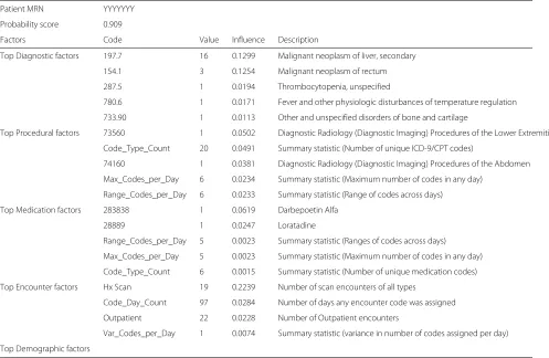
Table 5Prediction explanation generated on a random false positive patient with high probability score
Patient MRN YYYYYYY
Probability score 0.909
Factors Code Value Influence Description
Top Diagnostic factors 197.7 16 0.1299 Malignant neoplasm of liver, secondary
154.1 3 0.1254 Malignant neoplasm of rectum
287.5 1 0.0194 Thrombocytopenia, unspecified
780.6 1 0.0171 Fever and other physiologic disturbances of temperature regulation
733.90 1 0.0113 Other and unspecified disorders of bone and cartilage
Top Procedural factors 73560 1 0.0502 Diagnostic Radiology (Diagnostic Imaging) Procedures of the Lower Extremities
Code_Type_Count 20 0.0491 Summary statistic (Number of unique ICD-9/CPT codes)
74160 1 0.0381 Diagnostic Radiology (Diagnostic Imaging) Procedures of the Abdomen
Max_Codes_per_Day 6 0.0234 Summary statistic (Maximum number of codes in any day)
Range_Codes_per_Day 6 0.0233 Summary statistic (Range of codes across days)
Top Medication factors 283838 1 0.0619 Darbepoetin Alfa
28889 1 0.0247 Loratadine
Range_Codes_per_Day 5 0.0023 Summary statistic (Ranges of codes across days)
Max_Codes_per_Day 5 0.0023 Summary statistic (Maximum number of codes in any day)
Code_Type_Count 6 0.0015 Summary statistic (Number of unique medication codes)
Top Encounter factors Hx Scan 19 0.2239 Number of scan encounters of all types
Code_Day_Count 97 0.0284 Number of days any encounter code was assigned
Outpatient 22 0.0228 Number of Outpatient encounters
Var_Codes_per_Day 1 0.0074 Summary statistic (variance in number of codes assigned per day)
Top Demographic factors
was not diagnosed with XYZ, prescribed drug ABC, etc? This drop in log-probability is considered the influence the code has on the model’s decision for that patient. Demographic features are handled as follows. We zero out the age and swap the gender to the opposite sex, and measure the respective drops in probability. Finally we sort the codes in descending order by influence, and pick the top 5 in each code category. A random exam-ple of such a positive and false positive case are shown in Tables4and5.
Conclusion
We demonstrate that routinely collected EHR data can be used to create a system that prioritizes patients for fol-low up for palliative care. In our preliminary analysis we find that it is possible to create a model for all-cause mor-tality prediction and use that outcome as a proxy for the need of a palliative care consultation. The resulting model is currently being piloted for daily, proactive outreach to newly admitted patients. We will collect objective out-come data (such as rates of palliative care consults, and rates of goals of care documentation) resulting from the use of our model. We also demonstrate a novel method of generating explanations from complex deep learning models that helps build confidence of practitioners to act on the recommendations of the system.
Acknowledgments
We thank the Stanford Research IT team for their support and help in this project. Research IT, and the Stanford Clinical Data Warehouse (CDW) are supported by the National Center for Research Resources and the National Center for Advancing Translational Sciences, National Institutes of Health, through grant UL1 TR001085. The content of studies done using the CDW is solely the responsibility of the authors and does not necessarily represent the official views of the NIH. We thank Ziang Xie, and the anonymous reviewers for their helpful and insightful comments.
Funding
Publication costs were funded by grant GCDDG.
Availability of data and materials
Data used for this study is from Stanford University Clinical Data Warehouse, hosted by the Stanford Research IT.
About this supplement
This article has been published as part ofBMC Medical Informatics and Decision Making Volume 18 Supplement 4, 2018: Selected articles from the IEEE BIBM International Conference on Bioinformatics & Biomedicine (BIBM) 2017: medical informatics and decision making. The full contents of the supplement are available online athttps://bmcmedinformdecismak.biomedcentral.com/ articles/supplements/volume-18-supplement-4.
Authors’ contributions
SH and NHS envisaged the project. AA and KJ built the model and
implemented code, guided by LD, AN and NHS. All authors contributed to the writing of the manuscript. All authors have read and approved final manuscript.
Ethics approval and consent to participate
This work has obtained ethics approval by the Institutional Review Board of Stanford University under protocol 42078.
Consent for publication
Not applicable.
Competing interests
The authors declare that they have no competing interests.
Publisher’s Note
Springer Nature remains neutral with regard to jurisdictional claims in published maps and institutional affiliations.
Author details
1Department of Computer Science, Stanford University, Stanford, CA, USA. 2Center for Biomedical Informatics Research, Stanford University, Stanford, CA,
USA.3Department of Medicine, Stanford University School of Medicine,
Stanford, CA, USA.
Published: 12 December 2018
References
1. Where do americans die? Available: https://palliative.stanford.edu/home-hospice-home-care-of-the-dying-patient/where-do-americans-die/. Accessed 15 Apr 2017.
2. Dumanovsky T, Augustin R, Rogers M, Lettang K, Meier DE, Sean Morrison R. Special Report The Growth of Palliative Care in U.S. Hospitals: A Status Report. J Palliat Med. 2016;19(1):8–15.
3. palliative care, report card. 2015. Available:https://web.archive.org/web/ 20170316014732/https://reportcard.capc.org/#key-findings. Accessed 15 Apr 2017.
4. Spetz J, Dudley N, Trupin L, Rogers M, Meier DE, Dumanovsky T. Few Hospital Palliative Care Programs Meet National Staffing
Recommendations. Health Aff (Project Hope). 2016;9(9):1690–7. 5. Christakis N, Lamont E. Extent and determinants of error in doctors’
prognoses in terminally ill patients: prospective cohort study. BMJ Clin Res. 2000;320(7233):469–72.
6. most physicians would forgo aggressive treatment for themselves at the end of life, study finds. 2014. Available:https://med.stanford.edu/news/ all-news/2014/05/most-physicians-would-forgo-aggressive-treatment-for-themselves-.html. Accessed 15 Apr 2017.
7. Kutner JS, Steiner JF, Corbett KK, Jahnigen DW, Barton PL. Information needs in terminal illness. Soc Sci Med. 1999;48(10):1341–52.
8. Steinhauser KE, Christakis NA, Clipp EC, Mcneilly M, Grambow S, Parker J, Tulsky JA. Preparing for the End of Life: Preferences of Patients, Families, Physicians, and Other Care Providers. J Pain Symptom Manag J Pain Symptom Manage. 2001;2222:727.
9. Selby D, Chakraborty A, Lilien T, Stacey E, Zhang L, Myers J. Clinician Accuracy When Estimating Survival Duration: The Role of the Patient’s Performance Status and Time-Based Prognostic Categories. J Pain Symptom Manag. 2011;42(4):578–88.
10. Vigan ˙o A, Dorgan M, Bruera E, Suarez-Almazor ME. The Relative Accuracy of the Clinical Estimation of the Duration of Life for Patients with End of Life Cancer. Cancer. 1999;86(1):170–6.
11. Glare P, Sinclair C, Downing M, Stone P, Maltoni M, Vigano A. Predicting survival in patients with advanced disease. 2008;4:2.
12. White N, Reid F, Harris A, Harries P, Stone P, Pulenzas N. A Systematic Review of Predictions of Survival in Palliative Care: How Accurate Are Clinicians and Who Are the Experts? PLoS ONE. 2016;11(8):e0161407. 13. Macmillan DO. Accuracy of prediction of survival by different professional
groups in a hospice. Palliat Med. 1998;12:117–8.
14. Lau F, Downing GM, Lesperance M, Shaw J, Kuziemsky C. Use of Palliative Performance Scale in End-of-Life Prognostication. J Palliat Med. 2006;9(5):1066–75.
15. Karnofsky DA, Abelmann WH, Craver LF, Burchenal JH. The use of the nitrogen mustards in the palliative treatment of carcinoma.With particular reference to bronchogenic carcinoma. Cancer. 1948;1(4):634–56. 16. Pirovano M, Maltoni M, Nanni O, Marinari M, Indelli M, Zaninetta G,
Petrella V, Barni S, Zecca E, Scarpi E, Labianca R, Amadori D, Luporini G. A New Palliative Prognostic Score: A First Step for the Staging of Terminally Ill Cancer Patients for the Italian Multicenter and Study Group on Palliative Care. J Pain Symptom Manag Pirovano et al. 1997;17(4):231–9. 17. Knaus WA, Draper EA, Wagner DP, Zimmerman JE. APACHE II: a severity
of disease classification system. Crit Care Med. 1985;13(10):818–29. 18. Knaus WA, Wagner DP, Draper EA, Zimmerman JE, Bergner M, Bastos PG,
19. Le Gall J-R, Lemeshow S, Saulnier F. A New Simplified Acute Physiology Score (SAPS II) Based on a European/North American Multicenter Study. J Am Med Assoc. 1993;12(24):2957.
20. Cardona-Morrell M, Hillman K. Development of a tool for defining and identifying the dying patient in hospital: Criteria for Screening and Triaging to Appropriate aLternative care (CriSTAL). BMJ Support Palliat Care. 2015;3(1):78–90.
21. Fischer SM, Gozansky WS, Sauaia A, Min S-J, Kutner JS, Kramer A. A Practical Tool to Identify Patients Who May Benefit from a Palliative Approach: The CARING Criteria. J Pain Symptom Manag. 2006;31(4): 285–92.
22. Richardson P, Greenslade J, Shanmugathasan S, Doucet K, Widdicombe N, Chu K, Brown A. PREDICT: a diagnostic accuracy study of a tool for predicting mortality within one year: Who should have an advance healthcare directive? Palliat Med. 2015;29(1):31–7.
23. Horne BD, May HT, Muhlestein JB, Ronnow BS, Lapp˙e DL, Renlund DG, Kfoury AG, Carlquist JF, Fisher PW, Pearson RR, Bair TL, Anderson JL. Exceptional Mortality Prediction by Risk Scores from Common Laboratory Tests. AJM. 2009;122:550–8.
24. Cowen ME, Strawderman RL, Czerwinski JL, Smith MJ, Halasyamani LK, Cowen ME. Mortality predictions on admission as a context for organizing care activities. J Hosp Med. 2013;5(5):229–35.
25. Meffert C, R ˙ucker G, Hatami I, Becker G. Identification of hospital patients in need of palliative care-a predictive score. BMC Palliat Care. 2016;15. https://doi.org/10.1186/s12904-016-0094-7.
26. Ramchandran KJ, Shega JW, Von Roenn J, Schumacher M, Szmuilowicz E, Rademaker A, Weitner BB, Loftus PD, Chu IM, Weitzman S. A predictive model to identify hospitalized cancer patients at risk for 30-day mortality based on admission criteria via the electronic medical record. Cancer. 2013;6(11):2074–80.
27. Amarasingham R, Moore BJ, Tabak YP, Drazner MH, Clark CA, Zhang S, Reed WG, Swanson TS, Ma Y, Halm EA. An Automated Model to Identify Heart Failure Patients at Risk for 30-Day Readmission or Death Using Electronic Medical Record Data. Med Care. 2010;48(11):981–8. 28. Tabak YP, Johannes RS, Silber JH. Using Automated Clinical Data for Risk
Adjustment. Medical Care. 2007;45(8):789–805.
29. Makar M, Ghassemi M, Cutler D, Obermeyer Z. Short-Term Mortality Prediction for Elderly Patients Using Medicare Claims Data. Int J Mach Learn Comput. 2015;5(3):192–7.
30. Sim I, FH Z, SM T, SY H, N Z, Y H, M N. Two Ways of Knowing: Big Data and Evidence-Based Medicine. Ann Intern Med. 2016;164(8):562. 31. Obermeyer Z, Emanuel EJ. Predicting the Future - Big Data, Machine
Learning, and Clinical Medicine. N Engl J Med. 2016;9(13):1216–9. 32. Rose S. Mortality Risk Score Prediction in an Elderly Population Using
Machine Learning. Am J Epidemiol. 2013;3(5):443–52.
33. Wiemken TL, Furmanek SP, Mattingly WA, Guinn BE, Cavallazzi R, Fernandez-Botran R, Wolf LA, English CL, Ramirez JA. Predicting 30-day mortality in hospitalized patients with community-acquired pneumonia using statistical and machine learning approaches. J Respir Infect. 2017;1(3):5.
34. Motwani M, Dey D, Berman DS, Germano G, Achenbach S, Al-Mallah MH, Andreini D, Budoff MJ, Cademartiri F, Callister TQ, Chang H-J, Chinnaiyan K, Chow BJ, Cury RC, Delago A, Gomez M, Gransar H, Hadamitzky M, Hausleiter J, Hindoyan N, Feuchtner G, Kaufmann PA, Kim Y-J, Leipsic J, Lin FY, Maffei E, Marques H, Pontone G, Raff G, Rubinshtein R, Shaw LJ, Stehli J, Villines TC, Dunning A, Min JK, Slomka PJ. Machine learning for prediction of all-cause mortality in patients with suspected coronary artery disease: a 5-year multicentre prospective registry analysis. Eur Heart J. 2016;25(7):ehw188.
35. Cooper GF, Aliferis CF, Ambrosino R, Aronis J, Buchanon BG. An Evaluation of Machine-Learning Methods for Predicting Pneumonia Mortality. Artif Intell Med. 1997;9(2):107–38.
36. Vomlel J, Kružík H, Tma P, Pˇreˇcek J, Hutyra M. Machine Learning Methods for Mortality Prediction in Patients with ST Elevation Myocardial Infarction. In the Proceedings of The Nineth Workshop on Uncertainty Processing WUPES’12, Mariánské Láznˇe, Czech Republic. 2012. p. 204–213. 37. Avati A, Jung K, Harman S, Downing L, Ng A, Shah NH. Improving
palliative care with deep learning. IEEE; 2017. p. 311–316. Available:http:// ieeexplore.ieee.org/document/8217669/.
38. Lowe HJ, Ferris TA, Hernandez Nd PM, Weber SC. STRIDE – An Integrated Standards-Based Translational Research Informatics Platform. In: AMIA
Annual Symposium Proceedings. 2009. p. 391–5. Conference paper (AMIA Symposium).
39. LeCun Y, Bengio Y, Hinton G. Deep Learning. Nature. 2015;521:436–44. 40. Klambauer G, Unterthiner T, Mayr A, Hochreiter S Guyon I, Luxburg UV,
Bengio S, Wallach H, Fergus R, Vishwanathan S, Garnett R, (eds). Self-normalizing neural networks; 2017. p. 972–981. Curran Associates, Inc. Available: http://papers.nips.cc/paper/6698-self-normalizing-neural-networks.pdf. Accessed 2 Nov 2018.
41. Kingma DP, Ba J. Adam: A Method for Stochastic Optimization. In: Proceedings of the 3rd International Conference on Learning Representations (ICLR). 2014. Conference paper (ICLR). 42. Pytorch. Available:https://pytorch.org. Accessed 2 Nov 2018. 43. Pedregosa F, Varoquaux G, Gramfort A, Michel V, Thirion B, Grisel O,
Blondel M, Prettenhofer P, Weiss R, Dubourg V, Vanderplas J, Passos A, Cournapeau D, Brucher M, Perrot M, Duchesnay E. Scikit-learn: Machine learning in Python. J Mach Learn Res. 2011;12:2825–30.
44. He H, Garcia E. Learning from Imbalanced Data. IEEE Trans Knowl Data Eng. 2009;9(9):1263–84.
45. Davis J, Goadrich M. The Relationship Between Precision-Recall and ROC Curves. In: Proceedings of the 23rd international conference on Machine learning. 2006. p. 233–40. Conference paper (ICML).
46. Boyd K, Santos Costa V, Davis J, Page CD. Unachievable Region in Precision-Recall Space and Its Effect on Empirical Evaluation. In: Proceedings of the 29th International Coference on International Conference on Machine Learning Pages. 2012. p. 1619–26. Conference paper (ICML).
47. Yuan Y, Su W, Zhu M. Threshold-free measures for assessing the performance of medical screening tests. Front Public Health. 2015;3:57. 48. Manning CD, Raghavan P, Schütze H. Introduction to Information
Retrieval. New York: Cambridge University Press; 2008. Conference paper (KDD).
49. Ribeiro MT, Singh S, Guestrin C. Why Should I Trust You?: Explaining the Predictions of Any Classifier. In: Proceedings of the 22Nd ACM SIGKDD International Conference on Knowledge Discovery and Data Mining. 2016. p. 1135–44.