Complex Dynamics of the Chua’s Circuit System with Adjustable Symmetry and Nonlinearity: Multistability and Simple Circuit Realization

http://www.sciencepublishinggroup.com/j/wjap doi: 10.11648/j.wjap.20190402.12

ISSN: 2637-5990 (Print); ISSN: 2637-6008 (Online)

Complex Dynamics of the Chua’s Circuit System with

Adjustable Symmetry and Nonlinearity: Multistability and

Simple Circuit Realization

Nestor Tsafack

1, 2, *

, Jacques Kengne

1

1

Electrical Engineering Department, Institute of Technology Fotso Victor, University of Dschang, Bandjoun, Cameroon

2_{Department of Physics, Faculty of Sciences, University of Dschang, Dschang, Cameroon}

Email address:

*

Corresponding author

To cite this article:

Nestor Tsafack, Jacques Kengne. Complex Dynamics of the Chua’s Circuit System with Adjustable Symmetry and Nonlinearity: Multistability and Simple Circuit Realization. World Journal of Applied Physics. Special Issue: Symmetry and Multi-Stability in Simple Chaotic Systems and Circuits. Vol. 4, No. 2, 2019, pp. 24-34. doi: 10.11648/j.wjap.20190402.12

Received: July 25, 2019; Accepted: August 13, 2019; Published: September 11, 2019

Abstract:

Background: Since the invention of Chua’s circuit, numerous generalizations based on substitution of the nonlinear function have been reported. One of the generalizations is obtained by replacing the piecewise-linear with the cubic and/or quadratic polynomial. These nonlinearities are used to be implement using analog multipliers which are relatively expensive. In this realization we propose a different approach to synthetize both cubic and quadratic nonlinearities of empirical Chua’s circuit. Methods: The idea is to use diodes, Opamps and resistors to derive a PWL approximation of the cubic and quadratic functions. To demonstrate some complex phenomena observed in the system using the fourth order Runge-Kutta numerical integration method with a very small integration step. The bifurcation diagram which is the plot of local maxima of the temporal trace of a system’s coordinate as a function of the control parameter also constitutes an excellent tool for the study of dynamic systems. Results: The above mentioned standard nonlinear analysis tools have been exploited and it is found that the system with adjustable symmetry experiences a plethora of symmetric and asymmetric coexisting attractors. A particular feature of the system is related to the simplicity of the corresponding electronic analog circuit (no analog multiplier chip used to implement the cubic and quadratic nonlinearities). Conclusions: It is observed that the proposed Chua’s circuit system is more flexible (both symmetric and asymmetric) and displays complex dynamics behaviors of symmetric and asymmetric coexisting attractors. Note that this striking dynamic can be exploited in encryption algorithms.

Keywords:

Chua’s Circuit System, Adjustable Symmetry, Coexisting Bifurcations, Coexisting Attractors, Pspice Circuit Simulations

1. Introduction

Multistability of a dynamical system is usually taken to mean that there are coexisting attractors, each with a basin of attraction that depends crucially on the system’s initial values. The coexisting attractors can be stable equilibria, periodic cycles or strange attractors. There are even examples where all the three types of attractors coexist in phase space [1]. This striking dynamics has been previously observed in various dynamical systems including the Chua’s circuit [2-9]. Chua’s circuit is among the simplest electronic circuits characterized by chaos and many well-known nonlinear dynamic

function. Such an element is called the Chua’s diode. Note that the nonlinear function of the original Chua’s system is a continuous piecewise-linear function [18]. Since the invention of Chua’s circuit, numerous generalizations based on substitution of the nonlinear function have been reported [19-25]. One of the generalizations is obtained by replacing the piecewise-linear by the cubic and/or quadratic polynomial [24, 25]. In 1994, Zhong reported an implementation of Chua’s circuit with a smooth nonlinearity described by a cubic polynomial [25]. Note that this implementation is based on the utilization of three analog multipliers which are relatively expensive. Yang and coworkers investigated a modified Chua’s circuit system with both cubic and quadratic polynomials [24]. They focused on the chaos control by a delayed feedback method. The nonlinear function hyperbolic nonlinearity obtained from an active diode pair can be used to replace the Chua’s diode. For instance, Chen and collaborators reported hidden dynamics and multi-stability in an improved third order Chua’s circuit [26]. From the results of Chen, Bao and coworkers further investigated the coexistence of multiple attractors in Chua’s circuit and a plethora of point attractors, limit cycle attractors and strange attractors were found to coexist in phase space depending solely on the initial system’s values [1]. Memristor can also be used to replace the Chua’s diode in the original Chua’s circuit [27-29]. Cheng et al. reported a memristive bridge-based canonical Chua’s circuit by replacing the Chua’s diode with a first order memristive bridge diode [29]. They reported the complex nonlinear phenomena of coexisting bifurcations and coexisting attractors though the number of coexisting attractors depend crucially on the symmetry of the system. Symmetry always plays an important role in physical system. This property is found in a variety of system including nonlinear and chaotic systems [30-40]. Symmetric chaotic systems provide the possibility to observe coexisting attractors. Based on the nonlinear part of a symmetric system, the symmetry can be destroyed. A question can then be asked: what is the effect of an asymmetric nonlinearity on the multi-stable behavior of a system in general and on a Chua’s system in particular? In other word what are the mechanisms that occur when the Chua’s system loses its symmetry property in the multi-stable region? This question is very important since the answer lead to the generalization of multistability in the Chua’s system by adjusting its nonlinear part and hence its symmetry property.

In the present paper we investigated the coexisting bifurcations and coexisting attractors in a Chua’s system with adjustable symmetry and adjustable nonlinearity. The system is characterized by both cubic and quadratic nonlinear terms. Let us note that the quadratic nonlinearity is used to tune the symmetry of the whole system. A plethora of coexisting symmetric and asymmetric attractors can be found in the system’s parameter space. More important, the electronic analog circuit corresponding to the system under investigation is very simple. This is due to the fact that no analog multiplier is used to build the quadratic and the cubic polynomials.

2. Methods

2.1. Mathematical Formulation

Recently, Zhong investigated the implementation of Chua’s circuit with a cubic nonlinearity [25]. The circuit was modeled by:

3

1 2 1 1 1

2 1 2 3

3 2

( ) (a c )

x x x x x

x x x x

x x α α β  _{= − − +}  = − +   = −  & & & (1)

The method of practical implementation used to realize the cubic polynomial is interesting and can also be applied to implement Chua’s diodes with almost any smooth nonlinearity. However the main limitation is the presence of analog multipliers in the realization circuit of the cubic polynomial. In this paper we further investigate the dynamics of Chua’s system with both quadratic and cubic nonlinearities. The problem can be formulated as follows:

1 2 1 1

2 1 2 3

3 2

( ) _b( )

x x x f x

x x x x

x x α α β = − −   = − +   _{= −}  & & & (2)

Where f_b( )x₁ =ax₁+bx₁2+cx₁3 is a nonlinear polynomial containing cubic and quadratic nonlinearities which are implemented without any analog multiplier. More interesting, multistability in the symmetry boundary is discussed by switching the control parameter b given that the system is symmetric for b=0and becomes asymmetric forb≠0. A plethora of coexisting attractors are found in the systems parameters space. Throughout this work, unless otherwise mentioned, we assumed

β

=6.6 ; a= −1.16 ; c=0.06.

α

serves as the main bifurcation control parameter and bis used to tune the symmetry of the whole system as mention above.

2.2. Symmetry of the Model, Fixed Points and Stabilities

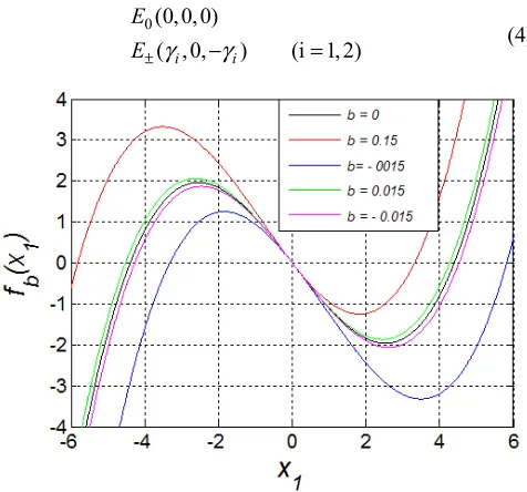
From system (2) it is obvious that by switching parameter b the symmetry of the model under investigation can be modified. Figure 1 is the representation of the nonlinear function f x_b( )where system’s symmetry breaks with the variation of parameter b. The curve in black is related to the particular case b=0. For this case the nonlinear function is symmetric and the system is invariant under the coordinate transformation ( ,x x x1 2, 3)⇔ − −( x1, x2,−x3) leading to

symmetric attractors, but in the general case this condition can only be achieved by switching parameter b related to the nonlinearity.

The fixed points of the proposed model (2) can be found by solving the following nonlinear system:

2 1 1

1 2 3

2

( ) ( ) 0

0

0 b

x x f x

x x x

From (3) it is obvious that system (2) has three equilibriums including one zero equilibrium point and two nonzero ones:

0(0, 0, 0)

( , 0,_{i i}) (i 1, 2)

E

E_±

γ

−

γ

= (4)

Figure 1. The nonlinear function f x for various values of the parameter k. b( )1

Notice that for b=0 the system displays two symmetric fixe points, but for

0

b≠ the later are no more symmetric.

Where γi are the solutions of the following third order

equation: (a 1)+ +b

γ

2+c

γ

3=0. The nonzero equilibrium

points E_±are symmetrical with respect to the origin E0 for

the particular case b=0. This symmetry is destroyed when 0

b≠ The Jacobian matrix at any equilibrium can be calculated as:

2

( a 1 2 3 0

1 1 1

0 0 b c J α µ µ α β  _{− − − −}    = −   ₋    (5)

With

µ

=0 for the zero fixed point; µ γ= i for the non-zero equilibrium points. The Eigen values related to the above matrix can be calculated for the particular case b=0 as follows:

0(0, 0, 0): 1 1.5307,

E λ

→ = +

2,3 0.8654 j1.6433

λ = − ±

1

2,3

( 1.633, 0, 1.633) : 2.5464, 0.1001 1.8652 E j

λ

λ

± → ± = − = + ± m (6)

Given that the real parts of these eigen values are positive and negative, the origin can be classified as unstable saddle point whereas the nonzero fixe points are unstable node-foci. Consequently the system displays self-excited strange attractors with the possibility of multistability in system (3). Similar calculations can be carried out in order to investigate the stability of the equilibrium points systems symmetry breaks (b≠0).

2.3. Numerical Methods

Numerical simulation plays a crucial role in predetermining the system’s parameters for its practical realization. To demonstrate the different phenomena observed in the system, the fourth order Runge-Kutta numerical integration method is used with an integration step 3

2 10

τ _{= ×} − _{. The solutions are} stored after the transient phase is discarded. The main indicator used to demonstrate the phenomenon of multistability is the coexisting bifurcation diagrams. Note these diagrams are obtained by plotting the local maximums of the variable x₃versus a given control parameter. Phase space trajectory plots are also used to illustrate the symmetric and asymmetric coexistence of attractors.

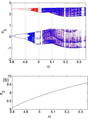
Figure 2. Systems dynamics for b=0; illustrating the coexisting bifurcation

diagrams obtained by switching parameter α when

6.6 ;a 1.16 ;c 0.06

β = = − = under three different initial conditions

(a) ( 1, 0 , 0) ; ( ) (20, 0 , 0)± b .

3. Results

3.1. Coexisting Bifurcations and Coexisting Attractors in the Particular Case (b=0)

To explore the coexisting behaviors with multistability in system (2) for the particular case b=0 , we fixed

6.6 ;a 1.16 ;c 0.06

β

= = − = and varied

α

in the range

4.8< <α 5.35. The system is solved under three different initial conditions (a) ( 1, 0 , 0) ; ( ) (20, 0, 0)± b leading to coexisting bifurcations (Figure 2).

with the initial value (1; 0; 0) . The corresponding bifurcation diagram is represented in black color. Various phase portraits are plotted for different values of the parameter

α

to illustrate the coexistence of point attractors, limit cycles and chaotic attractors (see Figure 5). Cross sections of the basin of attraction (Figure 3) with x1( )0 =0; x2( )0 =0 and x3( )0 =0 corresponding to the coexisting attractors are presented in Figure 5 (d).

To explore the different dynamic behaviors that

characterize system (2), we have also plotted the stability diagrams based on the Lyapunov exponent [41, 42]. These diagrams (Figure 4) highlight the different behavior zones according to the degree of stability (given by the maximal exponent of Lyapunov). Thus, Lyapunov exponents are unable to discriminate individual oscillatory phases. These graphs are of capital importance from a practical standpoint in that they give an overall idea of the dynamics under the effect of the parameters of the system.

Figure 3. Cross sections of the basin of attraction with x1( )0 =0; x2( )0 =0 and x3( )0 =0corresponding to the coexisting attractors presented in Figure 5.

(d).

3.2. Coexisting Bifurcations and Coexisting Attractors in the Particular Case (b≠0)

To investigate the multistability of system (2) in the symmetry boundary, We first fixe system’s parameters as b=0.015 (respectively b=0.015 )

β

=6.6 ;a= −1.16 ; c=0.06 and vary the control parameter

α

in the range4.8< <α 5.35. With these parameters the system is solved with various initial

conditions and coexisting bifurcations illustrated in Figure 6 are achieved. From these diagrams it is obvious that the coexisting attractors are no more symmetric. In light of Figure 6, a period-1 limit cycle can coexist with a period-2 one; a spiral chaotic attractor can coexist with a limit cycle and so on. Beside we have period doubling bifurcation (graph in blue and red colors) leading to different spiral chaotic attractor which are of different volumes. Several periodic windows intersect the chaotic region.

Figure 4. Lyapunov stability diagram in the (α, b), (β,b), (α β, ) planes illustrating the regions of periodic oscillations (λ ≤max 0) and the regions of chaotic

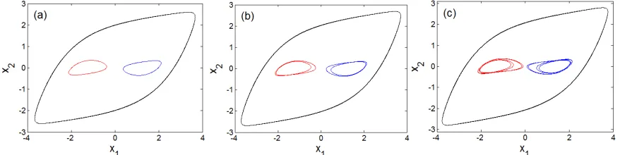
Figure 5. Coexisting attractors in the x1−x2plane when b=0 ; β =6.6 ;a= −1.16 ;c=0.06 (a)α=4.8, (b)α=4.85, (c)α=4.921, (d)α=4.967, (e)

4.915

α= , (f)α=5.23. Three different initial conditions are used (red−blue) ( 1, 0 , 0) ; (± black) (20, 0 , 0).

Figure 6. Systems dynamics for b=0.015 ; illustrating the coexisting bifurcation diagrams obtained by decreasing parameter α when

6.6 ;a 1.16 ; c 0.06

β = = − = under three different initial conditions

(a) ( 1, 0 , 0) ; ( ) (20, 0 , 0)± b .

For this set of parameter system (2) experiences the striking dynamics of coexisting bifurcations (see Figure 8) and thus coexisting attractors (see Figure 9). To the best author’s knowledge, multistability in the symmetry boundary has not yet been discussed in Chua’s system. Thus this work represents an enriching contribution to the understanding of the nonlinear dynamics of Chua’s oscillators. However, this striking phenomenon of disconnected coexisting attractors is also reported in other nonlinear dynamic systems such as Chua’s circuit [1-4], lazer system [43], chemical reaction [44], and the radio physical system [45], A special case where infinitely many attractors coexist, also referred to as extreme multistability is discussed by Hens and Wei [46-47].

Figure 7. Systems dynamics for b= −0.015; illustrating the coexisting bifurcation diagrams obtained by decreasing parameter α when

6.6 ;a 1.16 ; c 0.06

β = = − = under three different initial conditions

(a) ( 1, 0 , 0) ; ( ) (20, 0 , 0)± b .

Figure 8. Coexisting attractors in the x1−x2plane when b=0.015 β =6.6 ;a= −1.16 ;c=0.06 (a)α=4.8, (b)α=4.83, (c)α=4.91, (d)α=4.937, (e)

4.964

α= , (f)α=5.1. Three different initial conditions are used(red green)( 1, 0 , 0) ; (− ± blue) (20, 0 , 0).

Figure 9. Coexisting attractors in the x1−x2plane when b= −0.015 β =6.6 ;a= −1.16 ;c=0.06 (a)α=4.8, (b)α=4.83, (c)α=4.91, (d)α=4.937, (e) 4.964

α= , (f)α=5.1. Three different initial conditions are used(red−blue) ( 1, 0 , 0) ; (black) (20, 0 , 0)± .

3.3. Circuit Design and Spice Simulations

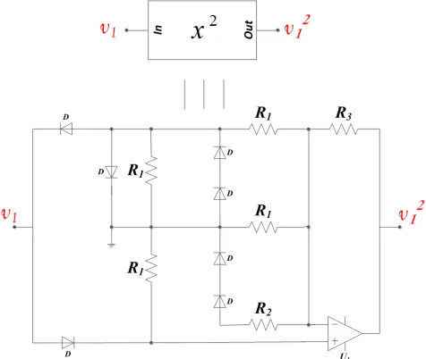
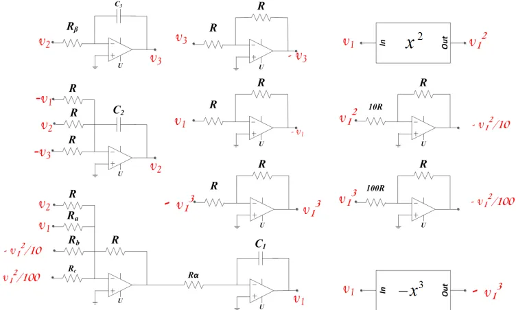
The aim of this section is to design and implement an analog computer for the experimental analysis of system (2). Note that system (2) contains both cubic and quadratic polynomials. These nonlinearities are used to be implemented using analog multipliers which are relatively expensive. In this realization we propose the use of an approach based on piecewise linear (PWL) functions [50-51]. In fact the idea is to use diodes, Operational amplifiers and resistors to derive a PWL approximation of the cubic and quadratic functions (see Figure 10).

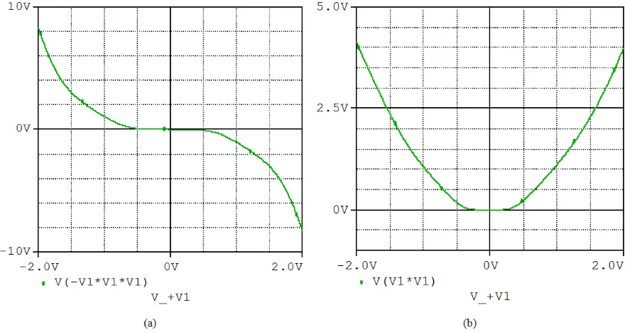
A circuit whose output is the square of the input signal is reported in Figure 10; while Figure 11 implements a PWL approximation of a circuit whose output is the cube of the input signal. Their transfer functions are represented in Figure 12 (a) and (b) respectively.

These circuits are more convenient for low cost realization and have been used to the Chua’s analog simulator presented in Figure 13 where the state variables x1, x2 and x3 of system (2)

are associated with the voltages v1, v2 and v3 across the capacitors C1, C2 and C3 respectively.

Figure 11. Circuital implementation of the cube function. Component values are the following: R1=200kΩ; R2=100kΩ; R3=12kΩ; R4= Ω2k ;

5 15 ;

R = kΩ R6=10kΩ..

Figure 12. Transfer function of the cube function (a) and the square function (b).

By applying Kirchhoff’s laws to the circuit of Figure 13, its nonlinear equations are derived in the following form:

2 3

1

1 2 1 1 1 1

2

2 1 2 3

3

3 2

1 1 1 1 1 1 1

( ) ( )

1

( )

1

e a b

e

e d C

dt R R R R R R R

d C

dt R

d C

dt R

α α

β

υ _{υ υ υ υ υ}

υ _{υ υ υ}

υ _υ



= − − + +

  

= − +

  

= − 



Figure 13. Electrical scheme of the analog calculator implementing the chaotic Chua’s system with asymmetric nonlinearity. The following Component values have been used to solve the circuit: R=10kΩ; C=10ηF; R_α= Ω2k ; R_β=1.52kΩ; Ra=62.5kΩ; Rb=66.66kΩ; Rc=1.66kΩ.

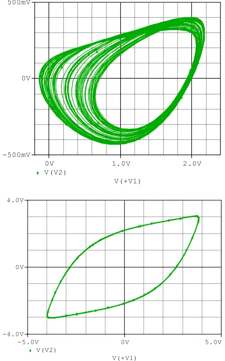
Figure 14. PSpice simulation results showing the coexistence of limit cycles for R_α=2.10kΩ; R_β=1.52kΩ; Ra=62.50kΩ; Rb=66.66kΩ;

1.66

c

R = kΩ: The initial conditions are (υC1(0),υC2(0),υC3(0))= ±( 2, 0, 0)

and (υC1(0),υC2(0),υC3(0))=(10, 0, 0).

V(+V1)

-2.0V -1.5V -1.0V -0.5V

V(V2) -400mV

0V 400mV

V(+V1)

0V 1.0V 2.0V

V(V2) -500mV

0V 500mV

V(+V1)

-5.0V 0V 5.0V

V(V2) -4.0V

0V 4.0V

V(+V1)

-2.0V -1.0V -0.0V

-2.4V V(V2) -400mV

Figure 15. PSpice simulation results showing the coexistence of two chaotic spiral attractors and limit cycles for R_α=2.03kΩ; R_β=1.52kΩ;

62.50 ;

a

R = kΩ Rb=66.66kΩ; Rc=1.66kΩ: The initial conditions are

1 2 3

(υC(0),υC(0),υC(0))= ±( 2, 0, 0)and (υC1(0),υC2(0),υC3(0))=(10, 0, 0).

Adopting the following rescale of time and variables:

; ( 1, 2, 3)

e i i T

t =tRC υ =x nV i= system (7) is identical to system (2) with the following definition of parameters:

; ; ; ;

a b c

R R R R R

a b c

R R R

α

R_α

β

R_β

= = = = = (8)

With the aim to confirm the theoretical results of section 3, i.e. the multistability in system (2), the circuit of Figure 14 is simulated using Pspice. R_α is used as the main control resistor and the rest of circuit components are fixed as:

1.52 ;

R_β = kΩ R_a =62.50kΩ; R_b =66.66kΩ; R_c =1.66kΩ. The agreement between the theoretical results (Figure 5) and Pspice simulations (see Figures 14, 15) shows the feasibility of the suggested chaotic system.

4. Conclusion

This paper has investigated the systematic analysis of a Chua’s circuit system. The adjustable symmetry of the system

is composed of both cubic and quadratic polynomials which have been implemented using PWL functions instead of analog multipliers. The stability analysis shows that the system has two stable nonzero fixed points. In addition the system is symmetric for the particular case (b=0). In this case the system displays complex nonlinear phenomena such as the symmetry breaking in which a symmetric pair of attractors coexists and merges into one symmetric attractor through an attractor-merging bifurcation. When b≠0the symmetry breaks down but its complex dynamics of multistability is revealed with the coexistence of limit cycles, chaotic spiral attractors and double scroll chaotic attractors. In contrast to the particular case (b=0), two asymmetric chaotic spiral attractors coexist and merge into one asymmetric double scroll chaotic attractor. For a kind of coexisting attractors the cross section of the basins of attraction of the various coexisting attractors has been plotted. More importantly, multistability in the symmetry boundary is discussed. Pspice simulation results support the numerical simulations. An experimental exploration of the parameter space of system (2) with application to image encryption deserves further studies.

References

[1] Bao B, Huagan W, Li X, Mo C. ‘‘Coexistence of Multiple Attractors in an Active Diode Pair Based Chua’s Circuit’’, International Journal of Bifurcation and Chaos, Vol. 28, No. 2 (2018) 1850019 (13 pages).

[2] Bao, B. C., Hu, F. W., Chen, M. & Xu, Q. [2015] “Self excited and hidden attractors found simultaneously in a modified Chua’s circuit,” Int. J. Bifurcation and Chaos 25, 1550075-1– 10.

[3] Bao, B. C., Jiang, P., Xu, Q. & Chen, M. [2016a] “Hidden attractors in a practical Chua’s circuit based on a modified Chua’s diode,” Electron. Lett. 52, 23–25.

[4] Bao, B. C., Li, Q. D., Wang, N. & Xu, Q. [2016b] “Multistability in Chua’s circuit with two stable node-foci,” Chaos 26, 043111.

[5] Chen, M., Yu, J. J. & Bao, B. C. [2015] “Hidden dynamics and multi-stability in an improved third order Chua’s circuit,” J. Eng. 87, doi: 10.1049/joe. 2015.0149.

[6] Chen, M., Xu, Q., Lin, Y. & Bao, B. C. [2017] “Multistability induced by two symmetric stable node-foci in modified canonical Chua’s circuit,” Nonlin. Dyn. 87, 789–802.

[7] Kengne J, Tsafack N, Kamdjeu L. Dynamical analysis of a novel single Opamp-based autonomous LC oscillator: antimonotonicity, chaos, and multiple attractors, International Journal of Dynamics and Control, 2018, https://doi.org/10.1007/s40435-018-0414-2.

[8] Lai Q, Tsafack N, Kengne J, Zhao XW. Coexisting attractors and circuit implementation of a new 4D chaotic system with two equilib) ria, Chaos, Solitons and Fractals 2018; 107: 92–102. [9] Guangya P. Fuhong M. Multistability analysis, circuit

implementations and application in image encryption of a novel memristive chaotic circuit, Non Dyn, 2017, DOI 10.1007/s11071-017-3752-2.

V(+V1)

0V 1.0V 2.0V

V(V2) -500mV

0V 500mV

V(+V1)

-5.0V 0V 5.0V

V(V2) -4.0V

[10] Wimol, S., Bandhit, S.: A simple RLCC-Diode-Opamp chaotic oscillator. IJBC 24, 1450155 (8 pages) (2014).

[11] Sprott, J.: Simple chaotic systems and circuits. Am. J. Phys. 68, 758-63 (2000).

[12] Matsumoto, Chua, L., Tanaka, S.: Simplest chaotic nonautonomous circuit. Phys. Rev. A 30, 1155-7 (1984). [13] Deane, J.: Modeling the dynamics of nonlinear inductor

circuits. IEEE Trans. 30, 2795-2801, (1994).

[14] Murali, K., Chua, L.: The simplest dissipative nonautonomous chaotic circuit. IEEE Trans. Circuits Syst. I. 41, 462-463 (1994).

[15] N. Tsafack and J. Kengne, “A particular class of simple chaotic circuits: Multistability analysis,” LAP LAMBERT Academie Publishing, ISBN: 978-613-9-46143-1, 2019.

[16] Christos, V., Akif, A., Pham, V., Ioannis, S., Ioannis, K.: A simple chaotic circuit with a hyperbolic sine function and its use in a sound encryption scheme. Nonlinear Dyn. 17, 3499 (9 pages) (2017).

[17] Kennedy, M.: Three steps to chaos-Part I: Evolution, IEEE Trans. On Circ. And Systems-I: Fundamental theory and applications, Vol 40, Oct 1993.

[18] Chua, L. O.: The genesis of Chuas circuit. Stuttgart: Hirzel-Verlag, AEU, 46, 250 (1992).

[19] Yu, L. M., V. L. Maistrenko: Cycles and chaotic Intervals in a time-delayed Chua’s circuit, Int. Jour. Bif. Chaos, Vol 3, 1993. [20] Bharathwaj M.: Memristor based chaotic circuit, IEEE

technical review, Vol 26, Issue 6, 2009.

[21] Leonov G. Kurnetsov N. Vagaitsev V. I.: Hidden attractor in smooth Chua system, Physica D, nonlinear phenomena, Vol 241, Issue 18, 2012.

[22] Bharathwaj M, Leon O Chua: Simplest chaotic circuit, IJBC, Vol 20, 2010.

[23] Kurnetsov N. V, Leonov G. A, Vagaitsev V. I: Analytical-numerical method for attractor localization of genelized chua’s system, IFAC Proceeding, doi: 10.3182/20100826-3-TR-4016.00009.

[24] Jihua Y., Liqin Z,: Bifurcation analysis and chaos control of the modified Chua’s circuit system, Chaos, Solitons and Fractals, 77 (2015) 332–339.

[25] Guo,-Qun Z.: Implementation of Chua’s circuit with a cubic nonlinearity, IEEE Transaction. On Circuit And Systems-I: Fundamental theory and applications, Vol 41, Dec 1994. [26] Chen, M., Yu, J. J. & Bao, B. C. [2015] “Hidden dynamics and

multi-stability in an improved third order Chua’s circuit,” J. Eng. 87, doi: 10.1049/joe. 2015.0149.

[27] Bao, B. C., Xu, Q., Bao, H. & Chen, M. [2016c] “Extreme multistability in a memristive circuit,” Electron. Lett. 52, 1008–1010.

[28] Bao, B. C., Yu, J. J., Hu, F. W. & Liu, Z. [2014] “Generalized memristor consisting of diode bridge with first order parallel RC filter,” Int. J. Bifurcation and Chaos 24, 1450143-1–4. [29] Chen M., Li M., Yu Q., Bao B?, Xu Q., Wang J.: Dynamics of

self-excited attractors and hidden attractors in a generalized

memristor-based Chua’s circuit, Nonlinear Dynamics (2015), 81, 215-226.

[30] Munmuangsaen B, Srisuchinwong B, Sprott JC. Generalization of the simplest autonomous chaotic system. Phys Lett A 2011; 375: 1445–50.

[31] Sprott JC. Elegant Chaos: algebraically simple flow. Singapore: World Scientific Publishing; 2010.

[32] Sprott JC. Simple chaotic systems and circuits. Am J Phys 2000; 68: 758–63.

[33] Sprott JC. A new chaotic jerk circuit. IEEE Trans Circuits Syst II Express Br. 2011; 58: 240–3.

[34] Eichhorn R, Linz SJ, Hanggi P. Simple polynomial classes of chaotic jerky dynamics. Chaos Solitons Fractals 2002; 13: 1– 15.

[35] Sedra S, Smith KC. Microelectronic circuits. London: Oxford University Press; 2003.

[36] Ozkurt N, Savaci FA, Gunduzalp M. The circuit implementation of a wavelet function approximator. Analog Integrated Circuits Signal Process 2002; 32: 171–5.

[37] Biswas D, Banerjee T. A simple chaotic and hyperchaotic time delay system: design and electronic circuit implementation. Nonlinear Dyn 2016; 83 (4): 2331–47.

[38] N. Tsafack, J. Kengne, ‘‘A Novel Autonomous 5-D Hyperjerk RC Circuit with Hyperbolic Sine Function ’’, Hindawi, The Scientific World Journal, Volume 2018, Article ID 1260325, 17 pages, https://doi.org/10.1155/2018/1260325.

[39] J. Kengne, S. Jafari, Z. T. Njitacke, M. Yousefi Azar Khanian, A. Cheukem, Dynamic analysis and electronic circuit implementation of a novel 3D autonomous system without linear terms, Communications in Nonlinear Science and

Numerical Simulation (2017), doi:

10.1016/j.cnsns.2017.04.017.

[40] Z. T. Njitacke, J. Kengne, L. Kamdjeu Kengne: Antimonotonicity, chaos and multiple coexisting attractors in a simple hybrid diode-based jerk circuit, Chaos, Solitons and Fractals 105 (2017) 77–91.

[41] Argyris J, Faust G, Haase M, Friedrich R. An exploration of dynamical systems and chaos, 2015.µ.

[42] Alombah NH, Fotsin HB, Kengne R. Coexistence of multiple attractors, metastable chaos and bursting oscillations in a multiscroll memristive chaotic circuit. Int J Bifurcation Chaos 2017; 27 (5): 1750067.

[43] C. Masoller ‘‘Coexistence of attractors in a laser diode with optical feedback from a large external cavity’’. Phys Rev A 50: 2569–2578, 1994.

[44] A. Massoudi, M. Mahjani, M. Jafarian, ‘‘Multiple attractors in Koper–Gaspard model of electrochemical’’. J Electroanal Chem 647: 74–86, 2010.

[45] A. Kuznetsov, S. Kuznetsov, E. Mosekilde, N. Stankevich, ‘‘Co-existing hidden attractors in a radio-physical oscillator’’. J Phys A Math Theor 48: 125101, 2015.

[47] Z. Wei, K. Rajagopal, W. Zhang, S. Takougang, A. Akgül ‘‘Synchronisation, electronic circuit implementation, and fractional-order analysis of 5D ordinary differential equations with hidden hyperchaotic attractors‘‘ Pramana – J. Phys. (2018) 90: 50, https://doi.org/10.1007/s12043-018-1540-2.

[48] X. Luo, M. Small, ‘‘On a dynamical system with multiple chaotic attractors’’. Int J Bifurc Chaos 17 (9): 3235–3251, 2007. [49] A. Pisarchik, U. Feudel, ‘‘Control of multistability’’. Phys Rep

540 (4): 167–218, 2014.

[50] A. Buscarino, L. Fortuna, Mattia Frasca, Gregorio Sciuto: A Concise Guide to Chaotic Electronic Circuits, SpringerBriefs in Applied Sciences and Technology, 2014, DOI 10.1007/978-3-319-05900-6.