Statistical mechanics analysis of LDPC coding in MIMO Gaussian channels

MIMO Gaussian Channels

Roberto C. Alamino and David Saad

Neural Computing Research Group, Aston University, Birmingham B4 7ET, UK

Abstract. Using analytical methods of statistical mechanics, we analyse the typical behaviour of a multiple-input multiple-output (MIMO) Gaussian channel with binary inputs under LDPC network coding andjoint decoding. The saddle point equations for the replica symmetric solution are found in particular realizations of this channel, including a small and large number of transmitters and receivers. In particular, we examine the cases of a single transmitter, a single receiver and symmetric and asymmetric interference. Both dynamical and thermodynamical transitions from the ferromagnetic solution of perfect decoding to a non-ferromagnetic solution are identified for the cases considered, marking the practical and theoretical limits of the system under the current coding scheme. Numerical results are provided, showing the typical level of improvement/deterioration achieved with respect to the single transmitter/receiver result, for the various cases.

1. Introduction

The statistical physics of disordered systems has been systematically developed over the past few decades to analyse systems of interacting components under different interaction regimes [1, 2]. It enables one to derive typical macroscopic properties of systems comprising a large number of units under conditions of quenched disorder, which correspond to different randomly sampled instances of the problem.

While their origin lies in the study of spin glasses [3, 4, 5], methods of statistical mechanics have been successfully employed to study a broad range of interdisciplinary subjects, from thermodynamics of fluids to biological and even sociological problems. In these studies, the problems were mapped onto known statistical physics models, such as Ising spin systems, and analysed using established methods and techniques.

In particular, these methods have been successfully employed recently to investigate hard computational problems [6, 7] as well as problems in information theory [8, 9] and multi-user communication [10]. They proved to be highly useful for gaining insight into the properties of the problems studied and in providing exact typical case results that complement the rigorous bounds reported in the theoretical computer science and information theory literature.

In the current study we employ the powerful analytical methods of statistical mechanics to examine the typical properties of Multiple-Input Multiple-Output (MIMO) communication channels where messages are encoded using state of the art Low-Density Parity-Check (LDPC) error correcting codes [11, 12, 13, 14].

MIMO channels are becoming increasingly more relevant in modern communication networks that rely on adaptive and ad-hoc configurations. Sensor networks, for instance, may rely on simultaneous transmission of information from a large number of transmitters that give rise to high levels of interference; while multiple access, at various levels, is exercised daily by millions of mobile phone users.

Communication over a MIMO channel is particularly amenable to a statistical physics analysis (see for example [15]) for the following reasons: firstly, previous studies in the areas of LDPC error-correcting codes [8] and Code Division Multiple Access (CDMA) [10, 16] paved the way for the study of MIMO systems; and secondly, the framework of multi-user communication channels is difficult to analyse using traditional methods of information theory [17], but can be readily accommodated within the statistical physics framework, particularly in the case of a large number of users. Previous results, derived via information theoretic approaches can be found for CDMA in [18, 19, 20, 21] and for the MIMO channel in [22].

2. The Model

LDPC codes, introduced by Gallager [11], are used to encode N-dimensional message vectors s into M-dimensional codewords t. They are defined by a binary matrix

A= [C1 |C2], calledparity-check matrix, concatenating two very sparse matrices known to both sender and receiver, with C2 (of dimensionality (M −N)×(M −N)) being invertible andC1of dimensionality (M−N)×N. The matrixAcan be either random or structured, characterised by the number of non-zero elements per row/column. Irregular codes show superior performance compared to regular codes [12, 23] if constructed carefully. However, to simplify the presentation, we focus on regular constructions; a generalisation to irregular constructions is straightforward [24, 25].

Encoding refers to the mapping of N-dimensional binary original messages s _∈

{0,1_}N _{to M-dimensional codewordst∈ {0,1}}M _{(M > N) by the linear product}

t=Gs (mod 2), (1)

with summations performed in the field _{0,1_} being indicated by (mod 2). The generator matrix has the form

G=

"

I C−1

2 C1 #

(mod 2) , (2)

where I is the N _×N identity matrix. By construction AG = 0 (mod 2) and the first

N bits of t correspond to the original message s.

Decoding is carried out by estimating the most probable transmitted vector from the received corrupted codeword [24, 8].

Here we analyse MIMO Gaussian channels withLsenders andO receivers in which each of L binary messages si ∈ {0,1}N_{, i = 1, ..., L, is encoded with an LDPC}

error-correcting code with an independently chosen parity-check matrix Ai into a binary codewordti ∈ {0,1}M_{. Messagessi and codewordsti are both vectors with two different}

indices, the bit index µand the sender/receiver index i. Boldface notation denotes the sets in the sender/receiver indices and the bit index is explicitly denoted. We concentrate on regular Gallager codes, with K non-zero elements per row andC non-zero elements per column in the parity-check matrix, obeying C = (1₋R)K, where R =N/M is the code rate. The codewords are transmitted in discrete units of time.

We use, for mathematical convenience, the map x _→ (₋1)x _{from the Boolean}

variables ti _{∈ {}0,1_}M _{onto spin variables ti ∈ {1,−1}}M_{. Although different, we denote}

both with the same letter ti; the appropriate use of each one being clear from the context. At each discrete time step µ, the (already mapped) vector tµ, µ = 1, ..., M is transmitted and corrupted by additive white Gaussian noise (AWGN) obeying

rµ=Stµ+νµ, (3)

where S is the O ×L interference matrix, which plays an essential role in the current analysis as it crosses messages between senders and receivers and is responsible for important interference effects. The time independent AWGN is given by the vector νµ= (νµ

1, ..., ν

µ

O) with ν µ

3. Replica Analysis

The statistical mechanics based analysis focuses on the decoding process as it is directly linked to the Hamiltonian within the physics framework [26].

Decoding is carried out as in LDPC error-correcting codes; the estimate of the first N bits of the codeword, which contain the original uncoded message, is made by introducing L dynamical variable values τi ∈ {±1}M_{, representing candidate vectors}

for each of the transmitted codewords and give rise to its corresponding estimates

{ti}, i= 1, ..., L, by the O receivers, each one having access to all received messages. In the statistical analysis, we are interested in the behaviour averaged over the system’s disorder, given by the quenched variablesr, all possible encodings (equivalently, all parity-check matrices Ai) and all transmitted codewords ti.

Allowing some degree of error in the decoding, in the form of a prior error probability, the bit error probability is minimised by the Marginal Posterior Maximiser (MPM) for each dynamical variable in τ = (τ₁, ..., τL) [27, 25].

ˆ

tiµ= sgnhτ_iµi_P(τ_|r₎. (4)

The expected overlap between the estimated and the transmitted codewords serves as a measure for the error correction performance

di = 1

M M

X

µ=1 D

tµ_isgnhτ_iµi_P(τ_|r₎ E

A1,...,AL,r,t

, (5)

where the average is taken over the joint probability distribution P(A1, ..., AL,r,t). Its value also indicates the dynamical transition from the ferromagnetic solution of perfect decoding to a non-ferromagnetic solution.

The free-energy in the thermodynamic limit M _{→ ∞} is given by

f =− lim

M→∞

1

βMLhlnZiA1,...,AL,r,t, (6)

where Z is the partition function

Z =X τ

exp

"

−β O

X

j=1

Hj(τ|r)

#

,

with the Hamiltonian component for each receiver j

Hj(τ|r) = 1 2σ2

j M

X

µ=1

rµ_{j −} L

X

i=1

Sjiτ_iµ

!2

. (7)

The Hamiltonian gives rise to a likelihood term for the agreement between the received aggregated vector and the candidate codewords. The decoding temperature β

is considered the same for every receiver and each τi obeys the parity-check constraint, which for the spin variables is defined by

M

Y

µ=1

The decoding process is aimed at maximising the probability

P(τ|r) = 1

Z exp

"

−β O

X

j=1

Hj(τ|r)

#

. (9)

To calculate f in the thermodynamic limit M, N _{→ ∞}, keeping the code rate

R =N/M constant, we use the replica method [1, 2] which relies on the identity

hlnZi= lim

n→0

∂lnhZn_i

∂n , (10)

and employs an analytical continuation of integer values of n to a real value that approaches zero. The calculations follow the same guidelines of [25] (see the appendix for further details). The partition function is given by

Z =X τ

" _L Y

i=1

χ(Ai, τi)

#

exp



−β

O

X

j=1

M

X

µ=1 1 2σ2

j

r_jµ− L

X

i=1

Sjiτ_iµ

!2

, (11)

with χ(Ai, τi) = 0 if τi does not obey the parity-checks in Ai and 1 otherwise. All Ai

are chosen from the same ensemble, meaning that all code rates are equal, Ri =R.

¿From information theoretical considerations, the capacity region is given by

αR < _C, where α _≡L/O is a characteristic constant of the system called its load and

C, the capacity with joint decoding for an arbitrary distribution of inputs, is obtained by conventional information theoretical methods [17] as

C = 1

2log2det(IO+SS

T_C−1

ν ), (12)

where T indicates transposition, IO is the O-dimensional unit matrix and Cν is an O -dimensional square diagonal noise matrix given by (Cν)jk =σj2δjk. This result will be

used as a benchmark and an upper bound for our results. In the following sections we compare the replica symmetric results with known information theoretical limits.

4. Single Transmitter

The case L = O = 1 is easily seen to recover the usual results for a simple Gaussian channel as obtained in [25]. In the particular case of one sender and an arbitrary number of receivers, the channel matrix is anO-dimensional column vector. The Replica Symmetric (RS) saddle point equations are (see Appendix A.1)

ˆ

π(ˆx) =

*

δ xˆ₋

K−1 Y

l=1

xl

!+

x

, (13)

π(x) =

*

δ x₋tanh

"_C−1 X

l=1

atanh ˆxl_+β O

X

j=1

rjSj σ2

j

#!+

ˆ x_,r

, (14)

where P(r) =QO

j=1N Sj, σj2

The overlap is given by

d =hsgn (ρ)iρ, with (15)

P(ρ) =

*

δ ρ−tanh

" _C X

l=1

atanh ˆxl+β O

X

j=1

rjSj σ2

j

#!+

ˆ x_,r

. (16)

The free-energy is

βf = C

K ln 2 +Chln(1 +xxˆ)ix,ˆx− C K

*

ln 1 +

K

Y

m=1

xm

!+

x

−

*

ln

( X

τ=±1 exp

"

− O

X

j=1

β

2σ2

j

(rj −Sjτ)2

# _C Y

l=1

1 +τxˆl )+

ˆ x_,r

. (17)

The ferromagnetic solution,

ˆ

π(ˆx) =δ(ˆx−1), and π(x) =δ(x−1), (18) represents perfect decoding; it exists for all noise levels and has free-energy f = O/2. The internal energy and the entropy can be derived by the well-known relations

u= ∂

∂β(βf), s =β(u−f). (19)

Let us study the symmetric case where all transmitters emit with the same unit power, all entries of S are equal to 1, and all receivers experience the same noise level

σ2_{. When equated to R, the capacity, derived from equation (12), gives the threshold} noise σ2

t corresponding to the Shannon limit of perfect decoding

C = 1 2log2

1 + O

σ2

=R ⇒ σ_t2 = O

22R/O ₋₁. (20)

To obtain numerical solutions for the various cases we iterated the saddle-point equations (13) using population dynamics and then calculated the quantities of interest such as the overlap d, the free energyf and the entropy s of equations (15)-(19).

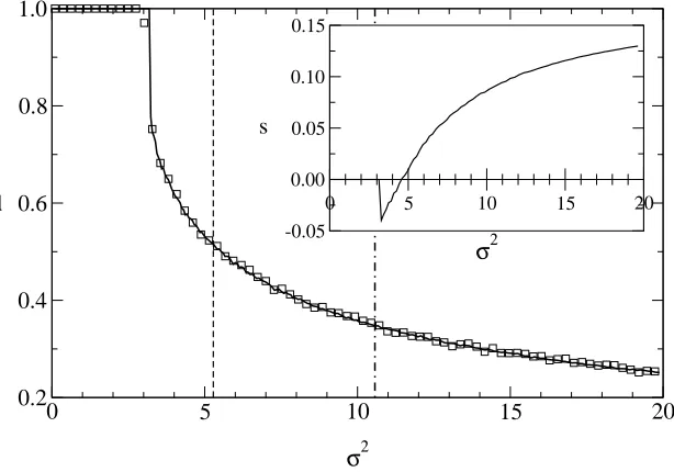
Figure 1 shows the overlap for L = 1 (one sender), O = 2 (two receivers), σ2

j =σ2

(equal noise level for all receivers) and R= 1/4 (withK = 4 and C = 3) at Nishimori’s temperatureβ = 1. The choice of Nishimori’s temperature simplifies the analysis as it is known that for it, the system does not enter the spin-glass phase [1]. Similar to the case of LDPC codes, there is no difference between the RS results using Nishimori’s condition and those obtained using the replica symmetry breaking ansatz for the channel studied here [28, 29]; this motivates our present choice of the replica symmetric ansatz.

0 5 10 15 20

σ2

-0.05 0.00 0.05 0.10 0.15

s

0 5 10 15 20

σ2

0.2 0.4 0.6 0.8 1.0

d

Figure 1. Overlap in the single-sender case for O _{= 2. The solid line describes} the result obtained by iterating the saddle point equations (13) from arbitrary initial conditions. The dotted-dashed line shows the theoretical limit obtained from equation (20) and the dashed line shows the theoretical limit for sending a doubled message via a single Gaussian channel. The squares correspond to results obtained using belief propagation with 20 different random parity-matrices and 100 corrupted codewords withM _{= 6000. The inset shows a plot of the entropy; the point where the} entropy becomes negative marks the emergence of metastable states and the dynamical transition point, while the point where it crosses back the zero entropy line marks the thermodynamical transition noise value.

The inset plot clarifies the type of solutions obtained as the noise increases: the entropy is zero up to the dynamical transition, meaning that the only stable state is the ferromagnetic one. Metastable suboptimal solutions emerge above this point and could be explored using replica symmetry breaking [28, 29]; they contribute to (unphysical) negative entropy values in this range [25]. The point where the entropy crosses the coordinate axis coincides with the thermodynamical transition, the later being always upper bounded by Shannon’s limit (vertical dashed line in the overlap plot).

The hollow squares, superimposed on the continuous line in the main plot, indicate the results of Belief Propagation (BP) averaged over 20 random constructions for the parity-check matrices and 100 corrupted codewords of length M = 6000. The minor disagreements, specially in the point of the dynamical transition, are due to finite size effects which disappear, although slowly, as the system size is increased. The message-passing algorithm is obtained in the same way as described in [24].

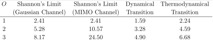
of the RS equations for O = 1,2,3 receivers. For O > 3 the numerical instabilities grow larger with O and a precise evaluation of the points is increasingly more difficult. The dynamical and thermodynamical transitions clearly occur always before Shannon’s limit. As expected, the more receivers, the higher the noise level tolerated by the system. However, the differences between the dynamical and the thermodynamical transition values, and between the later and Shannon’s limit, increase. Both are related to the fact that, in adding more receivers, the number of metastable states increases; they emerge earlier and contribute to a higher entropy.

Comparing the theoretical limit for sending a messageOtimes by a simple Gaussian channel and for the MIMO channel with one sender and O receivers, we see that the later is just O times the former. This can be understood noting that the information sent in the MIMO channel is the same as in the O-replicated Gaussian channel, but with O times the power; while in the MIMO channel, the O bits are sent with power 1 at each time step. We can see by the results that the transition points are even below the theoretical limit for the simple Gaussian channel and significantly below the MIMO limit. This clearly shows that in this type of communication channel, even with joint decoding, the available information is being poorly used. It makes a strong case for the use of network coding, i.e., to encode jointly the vectors tµ prior to transmission. Network coding, for instance using fountain codes [30, 31], is likely to make a better use of the resource by generating codewords that are more suited for better extraction of information under joint decoding.

Table 1. Comparison between the Shannon limit for a simple Gaussian channel and the MIMO channel, the dynamical transition point and the thermodynamical transition for the single-sender case (L_{= 1).}

O Shannon’s Limit Shannon’s Limit Dynamical Thermodynamical (Gaussian Channel) (MIMO Channel) Transition Transition

1 2.41 2.41 1.59 2.24

2 5.28 10.57 3.28 4.59

3 8.17 24.50 4.90 6.68

Another case of interest is the infinite number of receivers, O _{→ ∞}. The average over r’s in equation (13) can be substituted by an average over the Gaussian variable

v _≡ O

X

j=1

rjSj σ2

j

, (21)

which, for equal noise and Sj = 1, has zero mean and variance O/σ2 reflecting the

signal-to-noise ratio appearing in the capacity expression (20).

5. Multiple Access Channel

andσ2

j =σ2. Again, we find the threshold noiseσt2 by equating the capacity to the code

rate

C = 1 2log2

1 + L

σ2

=R ⇒ σ_t2 = L

22LR₋₁. (22)

Here, due to the interference effect in the received message, one must guarantee that the interference term has the correct order in L. Taking into account that the received messages are independent, we normalise their sum by the factor 1/√L.

The simplest case is L= 2 and the RS saddle point equations for user 1 are

ˆ

π1(ˆx1) = *

δ xˆ− K−1

Y

l=1

xl1 !+

x

, (23)

π1(x1) = *

δ x−tanh

(_C−1 X

l=1

atanh ˆxl₁+ βr

σ2√₂

+1 2ln





1₋tanh ₂β_σ2

tanhPC

l=1atanh ˆxl2+_σ2βr√₂

1 + tanh ₂β_σ2

tanhPC

l=1atanh ˆxl2+_σ2βr√₂

       + ˆ x,r , (24)

and the overlap is

d1 =hsgn (ρ)i_ρ, (25)

P(ρ) =

*

δ ρ−tanh

( _C X

l=1

atanh ˆxl₁+ βr

σ2√₂

+1 2ln





1₋tanh ₂β_σ2

tanhPC

l=1atanh ˆxl2+_σ2βr√₂

1 + tanh ₂β_σ2

tanhPC

l=1atanh ˆxl2+

βr σ2√₂

       + ˆ x,r , (26)

where _P(r) =_N √2, σ2

.

The corresponding set of equations for user 2 is identical to (23)-(26) except for interchanging the indices 1 and 2. The free-energy is given by

βf = C

K ln 2 + C

2 2 X

i=1

hln(1 +xixiˆ)_ix,xˆ− C 2K

2 X

i=1 *

ln 1 +

K

Y

m=1

xm_i

!+ x −1 2 * ln ( X

τ1,τ2 exp

"

− β

2σ2

r− τ1√+τ2

2

2# 2 Y

i=1

C

Y

l=1

1 +τixˆl_i )+

ˆ x_,r

. (27)

For the ferromagnetic solution (18), f = 0.25. Indeed, for the MIMO Gaussian channel studied here, we always have that the ferromagnetic free energy given by f = 1/2α.

0 2 4 6 8 10

σ2

0.10 0.15 0.20 0.25 0.30

Free energy Internal energy

0 5 10

-0.05 0.00 0.05 0.10 0.15

Figure 2. Free energy and internal energy in the MAC case for L _{= 2 represented} by the solid and dashed lines, respectively; the results have been obtained by iterating the saddle point equations (13) from arbitrary initial conditions. The dot-dashed line shows the theoretical limit obtained from equation (22) and the dotted line the thermodynamical transition point. The entropy as a function of the noise level is shown in the inset; the point where the entropy becomes negative marks the emergence of metastable states and the dynamical transition point, while the point where it crosses back the zero entropy line marks the thermodynamical transition noise value.

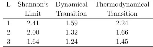
the crossing of the two energies and is denoted by the dotted line. The entropy function, shown in the inset plotted against the noise level, also helps to identify the dynamical and thermodynamical transitions (where the entropy becomes negative and where it crosses back the coordinate axis, respectively). Both points are below Shannon’s limit. Table 2 shows the results for L = 1,2,3 senders. The second column gives the theoretical limit obtained from equation (12); it shows the deterioration in performance as the number of senders increases, which is also evident in the results obtained by numerical results using the RS ansatz given by the dynamical transition (second column) and the thermodynamical transition (third column). Contrary to the single-sender case the difference between the transition points decreases with increasing L; this reflect the fact that additional inputs seem to increase the number of sub-optimal solution states (and hence reduce their free energy and affect the thermodynamical transition point) but have a lesser effect on the onset of the metastable states.

Table 2. Comparison between the Shannon’s limit, the dynamical transition point and the thermodynamical transition for the MAC case (O_{= 1).}

L Shannon’s Dynamical Thermodynamical Limit Transition Transition

1 2.41 1.59 2.24

2 2.00 1.32 1.66

3 1.64 1.24 1.45

transmitted information grows linearly with the number of transmitters; the capacity per user goes to zero in this limit, rendering the communication infeasible.

6. Channels with Interference

This section deals with a scenario where several transmitters send data simultaneously to an equal number of receivers; the transmission from a given transmitter to the corresponding receiver is corrupted by (small) deterministic interference from all other transmitters. The receivers can then communicate with each other to optimally extract the original messages. Some sensor networks are among the most well known examples of systems that could be modelled by this kind of channel.

In the following, we study two basic types of interference, the symmetric and the asymmetric cases. For simplicity, we limit the number of transmitters and receivers to

L=O = 2, making the interpretation of the results easier and more transparent. Both channels are depicted in figure 3. In the symmetric case, the transmitters send messages to both receivers (left picture) while in the asymmetric case only the first transmitter sends a message to the first receiver while the second transmitter sends to both.

Although the term interference channel is conventionally used when there is no cooperation between the receivers, the actual definition of this channel, as given in [17] for instance, does not explicitly exclude some information exchange between receivers. Therefore, the channels studied here can be viewed as instances of the interference channel where receivers cooperate to decode their messages by exploiting information gathered by other receivers to better estimate their own message.

Nevertheless, to avoid confusion and ambiguity we would like to point out that the channels with interference investigated here do not correspond to the conventional use of the term interference channel.

6.1. Symmetric Interference

We first study the case L=O = 2 with a symmetric interference matrix

S= 1 ǫ

ǫ 1

!

t

2

t

r

r

t

r

r

t

Symmetric Interference Asymmetric Interference

Figure 3. Diagram representing channels with symmetric (left) and asymmetric (right) interference. The first and second transmitters and receivers are denoted byt_1, t_2andr_1,r_{2, respectively. Arrows represent the transmitted messages and the double} line between the receivers indicatesjoint decoding.

where 0< ǫ_≤1. The capacity can be derived using equation (12) to obtain

C = 1 2log2

1 + 2(1 +ǫ 2₎

σ2 +

(1₋ǫ2₎2

σ4

. (29)

The RS saddle point equations are given by

ˆ

π1(ˆx1) = *

δ xˆ1−

K−1 Y

l=1

xl₁

!+

x

, (30)

π1(x1) = *

δ x1−tanh (_C−1

X

l=1

atanh ˆxl₁+ β

σ2√₂(r1+ǫr2)

+ 1 2ln





1−tanh(βǫ_σ2) tanh

β(ǫr1+r2)

σ2√₂ +

PC

l=1atanh ˆxl2

1 + tanh(βǫ_σ2) tanh

β(ǫr1+r2)

σ2√₂ +

PC

l=1atanh ˆxl2        + ˆ x_,r , (31)

where _P(ri) =_N (1 +ǫ)/√2, σ2

, i = 1,2. The corresponding equations for ˆπ2 and π2 are similar to those of ˆπ1 and π1 and are obtained by interchanging the indices 1 and 2. Here, the same scaling as in the MAC case is necessary due to the interference. However, for ǫ= 0, this scaling should be omitted as the interference vanishes, leaving two separate Gaussian channels.

The overlaps are given by

di =_hsgn (ρ)_iρ, (32)

P(ρ) =

*

δ ρ₋tanh

( _C X

l=1

atanh ˆxl₁+ β

σ2√₂(r1+ǫr2)

+ 1 2ln





1−tanh(βǫ_σ2) tanh

β(ǫr1+r2)

σ2√₂ +

PC

l=1atanh ˆxl2

1 + tanh(βǫ_σ2) tanh

β(ǫr1+r2)

σ2√₂ +

PC

l=1atanh ˆxl2        + ˆ x_,r . (33)

The free-energy f is

βf = C

K ln 2 + C

2 2 X

i=1

hln(1 +xixˆi)ix,xˆ−

C 2K 2 X i=1 *

ln 1 +

-1 -0.5 0 0.5 1 0

0.002 0.004 0.006

σ2=3.0

-1 -0.5 0 0.5 1

0 0.002 0.004 0.006

σ2=10.0

0 0.002 0.004 0.006

-1 -0.5 0 0.5 1

σ2=5.0

-1 -0.5 0 0.5 1

0 0.002 0.004 0.006

σ2=15.0

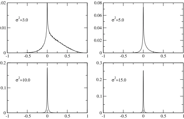
Figure 4. Profile of the π _{distribution. The plots are histograms with 500 bins for} a population of 40000 fields. The noise level valueσ2 _{is indicated in each graph. All} noise levels are above the dynamical transition point; below the transition point the distribution is a delta functionδ₍x_{−1). Note how the distribution changes slowly from} δ₍x_{−1) to} δ₍x_{) as the noise level increases.}

−1

2

*

ln

( X

τ1,τ2 exp

"

− β

2σ2

r1−

τ1 +ǫτ2

√

2

2

− β

2σ2

r2−

ǫτ1+τ2

√

2

2#

×

2 Y

i=1

C

Y

l=1

1 +τixˆl_i )+

ˆ x_,r

. (34)

Accordingly, the free-energy of the ferromagnetic solution (18) is f = 0.5, as for the simple Gaussian channel.

We solved numerically the saddle point equations (30) and calculated quantities of relevance in this case. The graphs for the overlap, entropy and energy are qualitatively the same as in the other two cases, with a similar behaviour with the appearance of both dynamical and thermodynamical transition points before Shannon’s limit.

-1 -0.5 0 0.5 1 0

0.01 0.02

σ2=3.0

-1 -0.5 0 0.5 1 0

0.02 0.04 0.06 0.08

σ2=5.0

-1 -0.5 0 0.5 1 0

0.1 0.2

σ2=10.0

-1 -0.5 0 0.5 1 0

0.1 0.2 0.3

σ2=15.0

Figure 5. Profile of the ˆπ _{distribution. The plots are histograms with 500 bins for} a population of 40000 fields. The noise level valueσ2 _{is indicated in each graph. All} noise levels are above the dynamical transition point; below it the profile distribution is simply a delta function δ_(ˆx_{−1). In this case, the profile changes abruptly from} δ_(ˆx_{−1) to an asymmetric distribution centred at ˆ}x_{= 0 and diverges rapidly to} δ_(ˆx₎ with the increasing noise.

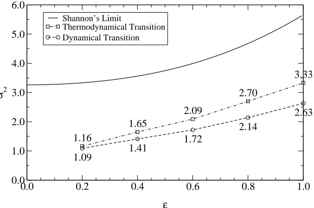
If one keep a constant code rate R = 1/4 but allows ǫ to vary, one obtains the dependence of the threshold noise as a function of ǫ, depicted in figure 6 (for β = 1,

K = 4 and C = 3). Both dynamical (dashed line) and thermodynamical transition values (dashed-dotted line) are upper bounded by the theoretical limit. Although this may seem counterintuitive, the communication resilience against noise increases with the interference level. This can be understood in the case of joint detection by noting that the increased interference provides more information about the other transmitters, such that higher levels of noise can be tolerated by joint decoding.

For largeO with L∼ O(1) or largeL with O ∼ O(1), the results should approach those obtained for large number of users in the single transmitter and in the MAC case, respectively. The behaviour must be dictated by the value of the system load α. In this case, we expect the results to cross from a behaviour similar to the one of a MAC channel for α >1 to one that resembles the single transmitter case for α <1. We are currently working on the analytical and computational aspects of this last case as well as on the case of largeO and L values while keeping the ratio L/O_{∼ O}(1) finite.

6.2. Asymmetric Interference

0.0 0.2 0.4 0.6 0.8 1.0 ε 0.0 1.0 2.0 3.0 4.0 5.0 6.0 σ2 3.33 2.70 2.09 1.65 1.16 2.63 2.14 1.72 1.41 1.09 Shannon’s Limit Thermodynamical Transition Dynamical Transition

Figure 6. Transition points and theoretical limits as a function of the interference level ǫ_{. The solid line represents the theoretical limit obtained from information theoretical} methods; the dashed-dotted and dashed lines correspond to the thermodynamical and dynamical transition points, respectively.

form (for L=O = 2)

S= 1 ǫ 0 1

!

, (35)

with 0< ǫ≤1. The corresponding capacity is now (again by (12))

C = 1 2log2

1 + (2 +ǫ 2₎

σ2 + 1

σ4

. (36)

The RS saddle point equations are given by

ˆ

πi(ˆxi) =

*

δ xiˆ − K−1

Y

l=1

xl_i

!+

x

, i= 1,2, (37)

π1(x1) = *

δ x1−tanh (_C−1

X

l=1

atanh ˆxl₁+ βr1

σ2√₂

+ 1 2ln





1₋tanh(₂βǫ_σ2) tanh

βǫr1

σ2√₂ +

βr2

σ2 +

PC

l=1atanh ˆxl2

1 + tanh(₂βǫ_σ2) tanh

βǫr1

σ2√₂ +

βr2

σ2 +

PC

l=1atanh ˆxl2        + ˆ x_,r , (38)

π2(x2) = *

δ x2−tanh (_C−1

X

l=1

atanh ˆxl₂+ βǫr1

σ2√₂+

βr2 σ2 + 1 2ln  

1₋tanh(₂βǫ_σ2) tanh

βr1

σ2√₂ +

PC

l=1atanh ˆxl1

1 + tanh(₂βǫ_σ2) tanh

βr1

σ2√₂ +

PC

l=1atanh ˆxl1        + ˆ x_,r , (39)

where P(r1) =N (1 +ǫ)/

√

2, σ2

In this case, the scaling 1/√L(although hereL= 2, the treatment can be extended to include a general number of sources) appears only in the first receiver, as it is being affected by the interference.

The overlaps are given by

di =hsgn (ρi)iρ_i, i= 1,2, (40)

P(ρ1) = *

δ ρ1−tanh ( _C

X

l=1

atanh ˆxl₁+ βr1

σ2√₂

+ 1 2ln





1−tanh(₂βǫ_σ2) tanh

βǫr1

σ2√₂ +

βr2

σ2 +

PC

l=1atanh ˆxl2

1 + tanh(₂βǫ_σ2) tanh

βǫr1

σ2√₂ +

βr2

σ2 +

PC

l=1atanh ˆxl2        + ˆ x_,r , (41)

P(ρ2) = *

δ ρ2−tanh ( _C

X

l=1

atanh ˆxl₂+ βǫr1

σ2√₂+

βr2 σ2 + 1 2ln  

1−tanh(₂βǫ_σ2) tanh

βr1

σ2√₂ +

PC

l=1atanh ˆxl1

1 + tanh(₂βǫ_σ2) tanh

βr1

σ2√₂ +

PC

l=1atanh ˆxl1        + ˆ x_,r , (42)

The free-energy f is obtained from

βf = C

K ln 2 + C

2 2 X

i=1

hln(1 +xixiˆ)_ix,xˆ− C 2K

2 X

i=1 *

ln 1 +

K

Y

m=1

xm_i

!+ x −1 2 * ln ( X

τ1,τ2 exp

"

− β

2σ2

r1−

τ1 +ǫτ2

√

2

2

− β

2σ2(r2−τ2) 2 # × 2 Y i=1 C Y l=1

1 +τixˆl_i )+

ˆ x_,r

, (43)

with the free energy of the ferromagnetic solutionf = 0.5.

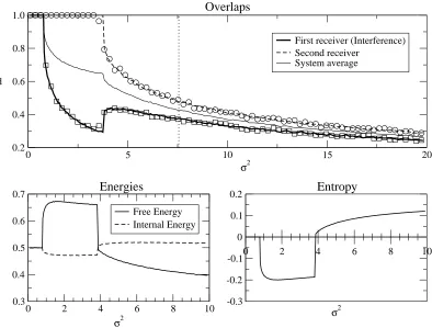
The numerical solution of (37) with ǫ = 1.0, β = 1 and R = 1/4 (K = 4, C = 3) leads to the results of figure 7. The top plot shows the overlaps for both receivers. Interestingly, the overlaps for the two receivers behave significantly differently in spite of the fact that messages are decoded jointly; a striking feature of the asymmetric case. The overlap for both receivers is 1 up to the point where the first receiver (thick continuous line), which experiences interference effects, exhibits a dynamical transition which signals the practical noise threshold for this system. The same point can be identified in the entropy plot (bottom right) as the point where the entropy becomes negative. This point is very far from Shannon’s limit (dotted line) σ2 _{≈ 7.56; this} can be explained by the additional metastable states introduced by the asymmetric interference. Note that the first receiver undergoes a (dynamical) transition before the second receiver (dashed line) that does not suffer from interference despite of the fact that the messages are decoded jointly.

levels, the first exhibits a suddenincreasein its decoding overlap. This behaviour may be understood by examining the average overlap, which can be viewed as the overlap for the entire system. The system’s overlap suffers a second transition at this point, although the average overlap continues to decrease monotonically; the system as a whole has a certain amount of retrievable information which keeps decreasing with the noise level.

The hollow squares and circles in the overlap plot show the results of BP simulations averaged over 10 random constructions for the parity-check matrices and 100 corrupted codewords of size M = 2000. Again, as in the case of the single transmitter (section 4), the BP solution is clearly in accord with the replica symmetric calculation. The small disagreements are due to noise and to finite size effects; they tend to disappear as the system size increases and the average is taken over a large number of realizations.

The result shows that information can be distributed among the receivers in a highly non-trivial way and also that for systems with many users, the thermodynamical transition is determined mostly by the weakest node (which experiences the highest levels of interference) and may lead to practical limits very far from Shannon’s bound.

7. Conclusions

We investigated the properties of coded Gaussian MIMO channels using methods of statistical mechanics. The problems investigated relate to the cases of a single transmitter, multiple access and interference in the case of multiple receivers and transmitters. In all cases, transmissions are coded using LDPC error-correcting codes.

The method used in the analysis, the replica approach, enables one to obtain typical case results that complements the theoretical bounds reported in the information theory literature. The numerical results obtained for particular MIMO channels and parameter values are presented and contrasted with information theoretical results.

MIMO channels are characterised by an interference matrix S which mixes inputs from the various transmitters to provide the messages at the receiving end. We examine cases where the interference matrix is deterministic. This requires the introduction of a non-trivial scaling in order to obtain meaningful results.

The results obtained provide characteristic, typical case, results in all cases. For the single transmitter and MAC cases we show both dynamical and thermodynamical transitions as functions of the number of receivers and transmitters, respectively. We see that the gaps between the practical and theoretical thresholds (dynamical and thermodynamical transitions, respectively), and the gap between them and Shannon’s limit, increase with the number of receivers for the single transmitter and decrease with the number of transmitters in the MAC case.

0 5 10 15 20

σ2

0.2 0.4 0.6 0.8 1.0

d

Overlaps

First receiver (Interference) Second receiver

System average

0 2 4 6 8 10

σ2

-0.3 -0.2 -0.1 0 0.1

0.2 Entropy

0 2 4 6 8 10

σ2

0.3 0.4 0.5 0.6

0.7 Energies

Free Energy Internal Energy

Figure 7. Numerical integration of saddle point equations for asymmetric interference. The upper plot shows the overlap for the first receiver (thick continuous line), which suffer the effects of interference, the second receiver (thick dashed line) and the average overlap for the entire system (thin continuous line). The Shannon limit for the system is depicted by the dotted vertical line. Squares and circles show the result of the corresponding BP-based simulations. At the bottom, the left graph shows the free-energy (continuous line) and the internal free-energy (dashed line) for the entire systems while the right graph shows the entropy values obtained under the RS ansatz.

level by averaging over a higher number of random independent noise sources.

The comparison with theoretical limits for the single transmitter case reveals an important feature of multiuser channels as to how the available information is used. The huge gap between the transition points and Shannon’s limit is indicative of a poor use of resource, and suggests network coding as a measure to achieve a better use of them; without it, the system’s efficiency remains below the achievable theoretical limit for sending the same message repeatedly via a simple Gaussian channel. One possible solution that we are currently investigating is the use of fountain codes [30, 31] for making a more efficient use of the available resource.

by the increase of (mixed) information in comparison to the noise level which can be decoded jointly, with an effectively lower noise level. The more moderate increase in the practical threshold (dynamical transition) is due to the difficulty in jointly decoding the various sources in practice due to the emergence of metastable states.

In the asymmetric case we found a striking different behaviour of the system. The new feature observed is the second transition suffered by the system as a whole. We also detected a surprising behaviour of the receiver which experiences interference; in spite of the joint decoding, the information available to it is suppressed by the second receiver. Only when the second receiver stops decoding perfectly, the performance of the first receiver improves.

An interesting extension, of significant practical relevance, would be the extend the LDPC coding framework to complex MIMO channels, where circular noise is considered [32]. Another possible extension is the case of a large number of senders and receivers where the ratio between them remains finite. The study of these and other related problems is underway.

Acknowledgements

Support from EVERGROW, IP No. 1935 in FP6 of the EU is gratefully acknowledged.

References

[1] Nishimori, H. Statistical Physics of Spin Glasses and Information Processing. Oxford University Press, Oxford, UK, (2001).

[2] M´ezard, M., Parisi, G., and Virasoro, M. Spin Glass Theory and Beyond. World Scientific Publishing Co., Singapore, (1987).

[3] Edwards, S. F. and Anderson, P. W. J. Phys. F: Metal Phys. 5, 965–974 (1975). [4] Sherrington, D. and Kirkpatrick, S. Phys. Rev. Lett.35, 1792–1796 (1975). [5] Kirkpatrick, S. and Sherrington, D. Phys. Rev. B17, 4384–4403 (1978). [6] Monasson, R. and Zecchina, R. Phys. Rev. Lett.76, 3881–3885 (1996).

[7] Hartmann, A. K. and Weigt, M. Phase Transitions in Combinatorial Optimization Problems: Basics, Algorithms and Statistical Mechanics. Wiley-VCH, (2005).

[8] Kabashima, Y. and Saad, D. J. Phys. A.37, R1–R43 (2004). [9] Murayama, T. J. Phys. A 35, L95–L100 (2002).

[10] Tanaka, T. IEEE Trans. Inform. Theory11, 2888–2910 (2002). [11] Gallager, R. IRE Trans. Info. TheoryIT-8, 21–28 (1962).

[12] Richardson, T., Shokrollahi, A., and Urbanke, R. IEEE Trans. on Info. Theory 47, 619–637 (2001).

[13] Richardson, T. and Urbanke, R. IEEE Trans. on Info. Theory47, 599–618 (2001).

[14] MacKay, D. Information Theory, Inference and Learning Algorithms. Cambridge University Press, Cambridge, MA, (2003). available at http://wol.ra.phy.cam.ac.uk/mackay/.

[15] de Miguel, R., Shental, O., Muller, R. R., and Kanter, I. J. Phys. A40, 5241–5260 (2007). [16] Tanaka, T. and Saad, D. Technical report, (2003). unpublished.

[17] Cover, T. and Thomas, J. Elements of Information Theory. John Wiley & Sons, New York, NY, (1991).

[19] Chung, J., Guo, F., Ng, S. X., and Hanzo, L. Vehicular Technology Conference 3, 1487–1491 (2003).

[20] Yue, G. and Wang, X. IEEE Trans. Wireless Commun.3, 1734–1745 (2004).

[21] Hoiu, J., Yi, Y., and Lee, M. H. EURASIP Journal onWireless Communications and Networking

1, 141–148 (2004).

[22] Sanderovich, A., Peleg, M., and Shamai, S. IEEE Trans. on Info. Theory51, 1437–1450 (2005). [23] Kanter, I. and Saad, D. Phys. Rev. Lett.83, 2660–2663 (1999).

[24] Vicente, R., Saad, D., and Kabashima, Y. InAdvances in Imaging and Electron Physics, Hawkes, P., editor, volume 125, 232–353. Academic Press (2002).

[25] Vicente, R., Saad, D., and Kabashima, Y. J. Phys. A33, 6527–6542 (2000). [26] Sourlas, N. Europhys. Lett.25, 159–164 (1994).

[27] Iba, Y. J. Phys. A32, 3875–3888 (1999).

[28] Franz, S., Leone, M., Montanari, A., and Ricci-Tersenghi, F. Phys. Rev. E66, 046120 (2002). [29] Migliorini, G. and Saad, D. Phys. Rev. E73, 026122 (2006).

[30] Luby, M. Inin Proc. of The 43rd Annual IEEE Symposium on Foundation of Computer Science, 271–282, (2002).

[31] Luby, M. G., Mitzenmacher, M., Shokrollahi, M. A., Spielman, D. A., and Stemann, V. InProc. of the 29th annual ACM symposium on Theory of computing, 150–159, (1997).

[32] Moustakas, A. L., Simon, S. H., and Sengupta, A. M. IEEE Transactions on Information Theory

49, 2545–2561 (2003).

Appendix A. Replica Symmetric Calculations

¿From the partition function (11), we can write the averaged replicated partition function _Zn≡ hZniA_1,...,AL,r_,t as

Zn= λ

M

2N L

X

{τa}

Z

dr exp



−

O

X

j=1

M

X

µ=1 1 2σ2

j

rµ_j − L

X

i=1

Sjiτ_iµ₀

!2



×exp



−

n

X

a=1

O

X

j=1

M

X

µ=1

β

2σ2

j

r_jµ₋ L

X

i=1

Sjiτiaµ

!2

 " _L

Y

i=1

Λi({τia})

#

, (A.1)

λ_≡ O

Y

j=1 (2πσ2

j)−1/2, (A.2)

where the multiplicative constants come from the normalisation of the probability distributions in the outside average and we defined τi0 ≡ti. Following [16], we have

Λi({τia})≡

* _n Y

a=0

χ(Ai, τia)

+

Ai

= 1

NA

I

DZi



 X

ωi

1

M

X

µ

Z_iµτ_iaµi

1 · · ·τ

µ iai

mi

!K



M−N

, (A.3)

where

DZi ≡

1 2M−N

n+1 M Y

µ=1

dZ_iµ

2πi

1

(Z_iµ)C+1, ωi ≡< a

i

and the variables mi assume all integer values for the index i from 0 to n+ 1. Defining

qωi ≡

1

M

X

µ

Z_iµτ_iaµi

1· · ·τ

µ iai

mi, (A.5)

and using integral representations for the delta functions, we can write

Zn= 2−N L

Z L

Y

i=1 Y

ωi

dqωidqωˆi

2πi/M !" _L Y i=1 X ωi

(qωi)

K

#M−N

× L

Y

i=1

exp ₋MX

ωi

qωiqωˆi

!

×X

{τa}

L

Y

i=1 "

I

DZiexp

X ωi ˆ qωi X µ

Z_iµτ_iaµi

1· · ·τ

µ iai

mi

!#

×λM

Z

dr exp

 − O X j=1 M X µ=1 1 2σ2

j

r_jµ₋ L

X

i=1

Sjiτ_iµ₀

!2

 ×exp  − n X a=1 O X j=1 M X µ=1 β

2σ2

j

rµ_j − L

X

i=1

Sjiτ_iaµ

!2

. (A.6)

Defining L Y i=1 Y ωi

dqωidqωˆi

2πi/M ≡DqDq,ˆ and γ ≡

2−(M−N)(n+1)₂−N

NA , (A.7)

and integrating over the variables Z_iµ, the µindices factorise and we obtain

Zn=

Z

DqDqˆexphMLf˜(q,qˆ)i, (A.8)

with

˜

f(q,qˆ)≡ 1

M lnγ+

(1₋R)

L L X i=1 ln " X ωi

(qωi)

K

#

− _L1 L

X

i=1 X

ωi

qωiqωˆ i+

1

Lln Φ, (A.9)

and

Φ≡λ

Z

dLr X

{τa}

  L Y i=1 1 C! X ωi ˆ

qωiτiai₁· · ·τiai_mi

!C

 ×exp  − O X j=1 1 2σ2

j rj₋ L X i=1 Sjiτi0 !2

 ×exp  − n X a=1 O X j=1 β

2σ2

j rj− L X i=1 Sjiτia

!2

Using the replica symmetric (RS) ansatz

qωi =q

i

0

(xi)mi−∆i

xi, xi ∼πi(xi),

ˆ

qωi = ˆq

i

0

(ˆxi)mi−∆i

ˆ

xi, xiˆ ∼πiˆ(ˆxi), (A.11)

where

∆i =

(

1, 0_{∈ {}ai

1, ..., aimi}

0, otherwise. (A.12)

For small n

ln

" X

ωi

(qωi)

K

#

= ln

2(q₀i)K

+n

*

ln 1 +

K

Y

m=1

xm_i

!+

x

, (A.13)

where _h·ix indicates the average over all variables x m i and

X

ωi

qωiqωˆi = 2q

i

0qˆ0i h

1 +n_hln(1 +xixiˆ)_ixi,ˆxii, (A.14)

X

ωi

ˆ

qωiτ

µ iai

1· · ·τ

µ iai

mi = ˆq

i

0(1 +τi0) * _n

Y

a=1

(1 +τiaxiˆ)

+

ˆ x

. (A.15)

Inserting the result in Φ and summing over the zero-th replicas we have

Φ =

2L_Qˆ

0 C

(C!)L

* X

{τa}

C Y l=1 n Y a=1 L Y i=1

1 +τiaxˆl_i

× exp  − n X a=1 O X j=1 β

2σ2

j rj − L X i=1 Sjiτia

!2

 +

r,ˆx

. (A.16)

where ˆQ0 ≡Q_iqˆ0i and P(r) = QO

j=1N

PL

i=1Sji, σ2j

. The sum over the n replicas factorises to

Φ =

2L_Qˆ

0 C

(C!)L

*( X

τ1,...,τL

C Y l=1 L Y i=1

1 +τixˆli

× exp  − O X j=1 β

2σ2

j rj− L X i=1 Sjiτi

!2

    n +

r,ˆx

. (A.17)

Appendix A.1. Single Transmitter

Let us consider L= 1. Then, for small n

ln Φ = ln(2ˆq0)

C C! +n * ln ( X τ C Y l=1

1 +τxˆl

exp " − O X j=1 β

2σ2

j

(rj −Sjτ)2

#)+

r,ˆx

. (A.18)

Appendix A.2. MAC

In this case, O = 1,

ln Φ = ln

2L_Qˆ

0 C

(C!)L

+n

*

ln

 

 X

{τi}

C

Y

l=1

L

Y

i=1

1 +τixˆl_i

exp



−

β

2σ2 r−

L

X

i=1

Siτi

!2

  

 +

r,xˆ

,(A.19)

and the corresponding extremisation, including the necessary normalisation, gives equations (23) of section 5.

Appendix A.3. Interference Channel

The case with L=O = 2 can be viewed as an interference Gaussian channel where the receivers cooperate to decode the received message. In this case

Φ =

4 ˆQ0 C

C!

*( X

τ1,τ2

C

Y

l=1

1 +τ1xˆl1

1 +τ2xˆl2

× e−2σβ2(r1−S11τ1−S12τ2)2_e−₂β_σ2(r2−S21τ1−S22τ2)2

onE

r,ˆx. (A.20)

Extremisation with respect to πi,i= 1,2 results in

ˆ

πi(ˆxi) =

*

δ xiˆ − K−1

Y

l=1

xli

!+

x

. (A.21)

Equating the functional derivative with respect to ˆπ1 to zero we obtain

π1(x1) =hδ(x1−h1(r,ˆx))ir,ˆx, (A.22)

where

h1(r,ˆx)≡ P

τ1,τ2τ1P

τ1τ2QC−1

l=1 1 +τ1xˆl1 QC

l=1 1 +τ2xˆl2

P

τ1,τ2P

τ1τ2QC−1

l=1 1 +τ1xˆl1 QC

l=1 1 +τ2xˆl2

, (A.23)

and