Considering the Light Nuclei in the Cluster Model from NU Method

(1)

2018; 3(4): 54-60

http://www.sciencepublishinggroup.com/j/wjap doi: 10.11648/j.wjap.20180304.11

ISSN: 2637-5990 (Print); ISSN: 2637-6008 (Online)

Considering the Light Nuclei in the Cluster Model from NU

Method

Sahar Aslanzadeh

1, *

, Mohammad Reza Shojaei

1

, Ali Asghar Mowlavi

2

1

Departement of Physics, Shahrood University of Technology, Shahrood, Iran

2_{Physics Department, Hakim Sabzevari University, Sabzevar, Iran}

Email address:

*

Corresponding author

To cite this article:

Sahar Aslanzadeh, Mohammad Reza Shojaei, Ali Asghar Mowlavi. Considering the Light Nuclei in the Cluster Model from NU Method.

World Journal of Applied Physics. Vol. 3, No. 4, 2018, pp. 54-60. doi: 10.11648/j.wjap.20180304.11

Received: September 9, 2018; Accepted: September 27, 2018; Published: January 23, 2019

Abstract:

In this work, the energy levels of light nuclei from the NU method are calculated and their structures are determined. Therefore, by using a local potential that is suitable for light nuclei and compatible with the Hafstad-Teller potential, the Schrodinger equation from NU method is solved and the energy levels and wave functions are obtained. For more accuracy, the spin-orbit and tensor potentials are added to the central potential as perturbation and the first-order energy correction is obtained for the different states of many alpha systems. So, we calculate the energy levels of nuclei 8Be and 16O

and compare the obtained results with the experimental data and get a good agreement. This agreement is better for 16O than 8

Be. Therefore, anybody can conclude that the α cluster model has the better results for the nuclei with the number of more alpha particles. Finally, by the strength of Coulomb’s repulsion, it is shown that the ground and first excited states of the 16O

nucleus have the tetrahedral and square configurations, respectively. Also, it is obtained that the structures of the second and third excited states are as square and linear chain that these structures show the non-localized gas configuration for the higher excited states of 16O nucleus.

Keywords:

Cluster Model, NU Method, Structure of Nuclei, Energy Levels

1. Introduction

In all branches of physics, usually, the construction of a suitable model compatible with experiment, is very important for solving the physical problems. In the nuclear physics, because of the complexity of the force between nucleons, it is suitable to find a model to decrease these complexities. One of these models is the cluster model. This model is based on this assumption that the nuclei can be considered as the small clusters of nucleons that the most important cluster is the alpha particle, i.e. the nucleus of 4He. This model was created after the decay of alpha particles from the heavy nuclei like the radionuclides and this topic was expressed that probably the nuclei have been composed of the alpha particles [1]. Therefore in the past decades, a number of nuclei have been considered as the many-alpha systems. From the point of view the nuclear structure, the alpha decay is represented as the particle decay from a virtual nuclear level. The experimental results show that the nuclei with A >

150 are often more unstable than the alpha decay and for the very light nuclei, the probability of alpha decay is very low [2]. However, this model has the better results for light nuclei, especially for the nuclei with the full layers, such as and [3-11]. On the other hand, in the light nuclei, deviation from the spherical state is interpreted as the cluster structure of these nuclei.

(2)

clusters is the basis of the nucleus movement.

So the article is organized as follows: Sec. II is started by introducing a local potential that is suitable for the light nuclei. According to this potential and using an appropriate approximation, the Schrodinger equation is solved through the NU method. In this section, the energy levels and the wave functions are obtained for a two-body system. Also, the spin-orbit and tensor potential as the perturbation terms are added to obtain the energy levels with higher accuracy.

In Sec. III, the light nuclei of and are considered and energy levels of these two nuclei are obtained. These results are compared with the experimental data and the structure of nucleus in different states is determined. Finally, in Sec. IV, the results of paper are written.

2. Solutions of the Schrodinger Equation

Using the NU Method with a Local

Potential

In this section, the energy levels and wave functions are obtained from the Schrodinger equation using a local potential from the NU method. This potential is selected by the Hafstad-Teller potential [21-27]. One of the best potentials for the light nuclei is the Ali-Bodmer potential [28, 29] which is compatible with the Hafstad-Teller potential. Therefore, a local potential similar to the Ali-Bodmer potential is considered for this work as a central potential. This potential is as:

= + = − + + ,

(1)

where = ! and = ! . The , , ! and

! are the attractive depth, the repulsive depth, the range of the attractive and repulsive sections, respectively. _" is the strength of Coulomb’s repulsion calculated from the Coulomb’s potential. In this potential, the first two terms are or the local potential between the alpha particles. In the above potential, the repulsive part at small distance results from the Pauli exclusion principle and the attraction part at large distances is for the Van Der Waals potential [30]. Although the internal structure of the alpha particles can be ignored [31-34], but according to the repulsive part of this potential, the effects of Pauli exclusion principle are somewhat considered. Now, for higher accuracy, we exert the contribution of spin and isospin as the spin-orbit term and the tensor term in the total potential and consider these terms as the perturbation potentials because the values of these terms are very small compared to the central potential. So the potential totally is as:

= + #.% &. ' + ( ' . (2) Now in this stage, the radial portion of Schrodinger equation is solved with the central potential from the NU method and finally the terms of spin-orbit and tensor are applied as the perturbation potential at the energy levels. The radial portion of the Schrodinger equation is written as:

)** _{+ )}* ₊ +

ℏ -. − −

ℏ / /0

+ 1 ) = 0, (3) where µ, l, E and R(r) are the reduced mass of clusters, the quantum number of angular momentum, the total energy of the system and the radial section of the wave function, respectively. Substituting Eq.(1) into Eq.(3), we get:

)** _{+ )}* ₊ +

ℏ 3. − − + + −

ℏ / /0

+ 4 ) = 0. (4)

The above equation can be written as:

5

5 +

5

5 + 67

8

− 7 8 − 79 − 7 +

: ; ) = 0, (5)

where the parameters of it are as follows:

7 = +_ℏ , 7 = +_ℏ , 79= +_ℏ <, 7 = = = + 1 , ? = _ℏ+@. (6)

Because Eq.(5) cannot be solved using analytical methods, so the exponential functions in this equation should be approximated. This approximation is up to degree at most two of the variable r, because the VN (r) potential, i.e. the potential between alpha particles which is due to the potential between the nucleons, is short-range(1fm). I.e. the potential of VN(r) at r > 1fm can be ignored. Then, ratios _A and _A are less 0.5, and degree after 2 is the 4th grade that the previous ratios to the power 4 are negligible. Therefore, this approximation is a good approximation and degree 2 of r is suitable for the NU method. So, Eq.(5) is simplified as:

5

5 +

5

5 + BC

D

A + ? E + 7 − 79 − 7 +

7 F ) = 0. (7)

For simplification, the parameters α, β and γ are defined as:

! = − C_AD + ? E،G = 7 − 7₉،H = 7 + 7. (8)

So considering these parameters and the change of variable r → s and the equivalence ψ (r) ≡ R(r), Eq.(7) is converted to:

5 I J

5J +J

5I J

5J +J K−!L + GL − HMN L = 0. (9) Comparing the above second order differential equation with the equation of hypergeometric-type NU, i.e. the below equation [35,36]:

N** _{L +}OP J

Q J N* L + QR J

(3)

Somebody can get:

S̃ = 2, σ s = s, σR = −αs + βs − γ. (11) Now from the NU method, one can solve Eq. (9). From Eq.(10), the important function π (s) [35] can be obtained:

[ L =Q\J 8OP J ± ^_Q\J 8OP J` − aP L + ?a L . (12)

Since π(s) should be a polynomial of degree at most one, so the discriminant of the term under the square root sign in the above equation is zero. Solving this equation, one can get values of k. By calculating k and using the equation below:

π L = KS L − S̃ L M, (13)

the function τ (s) is obtained as:

S L = 1 + b1 + 4H − 2√αs. (14) After calculating function τ (s), one can obtain λ from k = λ − π ′ (s) and e_f from the equation below:

λ_f= −gS* L −f f8 a** L , g = 0,1,2,3, …. (15)

So the two parameters λ and e_f are as follows:

e = G − b! 1 + 4H − √α,λ_j= 2n√α (16) From equality of λ and e_f, anyone can get:

! = l

m 0 f0b 0nop. (17) Substituting Eqs. (5) and (7) into Eq. (16), the low equation is obtained:

. = − − ℏqmr A 8 <p s 0 f0t 0nu vwrxyx_ℏ 0z z0 {|

, (18)

where this equation is the eigenvalues of energy of the two cluster nuclei for a local potential. Let us now turn attention to find the radial wave functions for this potential. Taking the wave function ψ (s) as ψ (s) = ϕ (s) }_f L and substituting this function into Eq.(9), somebody can get:

σ L }** L + S L }* L + e} L = 0, (19) where

~\ J ~ J

=

• J

Q J

,

(20)

and

}f L =_{‚ J}€• 5 •

5J•Kaf L ƒ L M. (21) The function }_f L in the above equation is solution of Eq. (19) called Rodrigues relation. In this relation, _f and ρ(s)

are the normalization constant and the weight function, respectively. ρ(s) must satisfy condition[35,36]:

_a L ƒ L `*= S L ƒ L . (22)

Now using Eqs. (11), (13) and (14) into Eq. (20), „ L is gotten as:

„ L = 8√AJ_L…b 0no8 _,₍₂₃₎ and substituting Eqs. (11) and (14) into Eq.(22), one can obtain:

ƒ L = 8 √AJ_Lb 0no_,₍₂₄₎ for the weight function ρ(s). Considering the above equation for ρ(s), the function }_f L in Eq.(21) is written as:

}f L = f √AJL8b 0no 5

•

5J•_ 8 √AJLf0b 0no`. (25) Now we can obtain the wave function ψ(s) from ψ(s) = ϕ(s) }_f L as

N L = f √AJL8

…_{mb 0no0 p 5}•

5J•_ 8 √AJLf0b 0no`. (26) Using the generalized Laguerre polynomials:

&f † =‡ ˆ f!

5•

5‡• 8‡ †A0f , (27) the function ψ(s) is rewritten in terms of &A_f † as follow:

N L = f 8√AJL

…_{mb 0no8 p}

&fb 0no m2√! Lp, (28) Where _f is the normalization constant. For calculating f, using the normalization condition, Š ‹ ) Œ = 1 and orthogonality relation of the generalized Laguerre polynomials, Š †‹ A0f 8‡&A_f † &A_• † Œ† = f0A !_f! 2g +

! + 1 Žf,•, one can get:

f= t f!m √Ap

√…••‘•

f0b 0no0 mf0b 0nop!. (29)

So the radial wave function of the Schroedinger equation is as:

) =

t_{m f0b 0no0 pmf0b 0nop!}f!m √Ap√…••‘• 8√A …mb 0no8 p_& f

b 0no _{m2√! p.}₍₃₀₎

(4)

Therefore the value of the first-order perturbed energy correction in the state |n > is determined by:

.f =< g“ #.% &. ' + ( '” “g > =

Š Nf ∗ m #.% &. ' + ( '” pNf Œ , (31)

where N_f is the unperturbed wave function for the central potential. By equivalence N_f ≡ ) and using Eq. (30), value of ._f can be calculated.

3. Clustering Examples

3.1. The Nucleus ™˜š

The simplest example for cluster structure of the nuclei is the nucleus which is constructed from the two alpha particles. This nucleus is totally unstable in the ground state and decays to the two alpha particles by 92KeV. In the potential of Eq. (1), values of parameters for this nucleus should be determined. The parameter µ of this nucleus is as •

that is equal to 1876ž_Ÿ . Also, the value of _" is

obtained by the Coulomb’s potential which is 4 for this nucleus. Therefore, for nucleus, _" is equal 5.76MeV.fm that = 1.43998MeV.fm. Also, the other parameters have been gotten by fitting the ground state and the first excited state of the nucleus to the experimental data. In this way, the parameters ¡ , , ! , and ! for the nucleus in Eq.(1) are obtained as 33.101MeV, 50.22MeV, 3.33fm, 2.5fm, respectively[37]. Because the nucleus has two particles, So one can use Eqs. (18) and (30) to calculate the energy levels, i.e. . , and the wave function of nucleus . Also, by using Eqs. (31) and (30) for this nucleus, the value of corrected energy, i.e. ._f , is calculated which is equal to zero when the system is in the zero spin. For example, the value of ._f for the 00 state is equal to zero, but this value for the 20 state is equal 2.35MeV. We calculate the value of

.f for the second excited state, i.e. 40, equal to 4.15MeV. Therefore the calculated results for the central potential and perturbed potentials along with the experimental data have been shown in Table (1).

Table 1. The energy levels of nucleus .

The levels ¢_£ ¤š¥ ¢_£+ ¢_¦§ ¤š¥ ¢š¨© ¤š¥ ª«, ¬, -, ®

The ground state -57.74 -57.74 -56.50 00, 0, 0, 0

The first excited state -54.94 -52.92 -53.47 20, 0, 2, 1

The second excited state -53.42 -49.27 -44.80 40, 0, 4, 1

3.2. The Nucleus of §¯°

Because the number of alpha particles in the nucleus is more than two, so this many-particle system can be made from a variety of geometric arrangements of four alpha particles. Therefore the structure of the ground state of this nucleus should be influenced by clustering or its symmetries. Now we have to see which one of the α cluster configurations in has the lowest energy. The various calculations show that the tetrahedral structure is the form of the ground state which challenges the traditional shell model picture [38-40]. In this section, we also consider the structure of the ground state of the nucleus by the Coulomb’s potential. The excited states of this nucleus may evolve into the square, or linear chain, or non-localized gas configuration [39-41]. For investigating this four-body system, the Jacobi coordinates are used that are ± , ± , ±₉ and R, the center of mass as:

± = ²…8 ²

√ , ± =

²…0 ² 8 ²³

√ , ±9=

²…0 ² 0 ²³89 ²•

√ , ) =

²…0 ² 0 ²³0 ²•_,₍₃₂₎

where ² , ² , ²₉ and ²_n are the relative positions of the four

particles in nucleus. In the many-particle systems, the mathematical formulations can be simplified by the Jacobi coordinates. Now the hyper-angles ´ , ´ and the hyper-radius quantity x are introduced as[42-44]:

† = b± + ± + ±9, Ѳ = tan8 _ ¸_¸…` , Ѳ = tan8 b¸…_¸0¸_³ .(33)

The Schrodinger equation in Eq. (8) for the N-Body systems in terms of the hyper-radius quantity x is:

5 I ‡

5‡ +

¹8 ‡

5I ‡

5‡ +‡ K−!† + G† − HMN † = 0, (34) where D=3N-3 and N is the number of particles. In here, Eqs. (17) and(29) are written as:

. = − − ℏqmr A 8 <p

s 0 f0t 8¹ 0nu qºr_ℏ 0/ /0 {|

, (35)

and

) = t_{_ f0b 8¹ 0no0 `_f0b 8¹ 0no`!}f!m √Ap^ » ••‘• 8√A …_b 8¹ 0no8 `_& f

b 8¹ 0no _{m2√! p.}

(36)

In order to calculate energy levels, parameters of potential like the nucleus should be determined. First, we consider _", i.e. strength of the Coulomb’s repulsion. If the ground state structure of nucleus is the tetrahedral

(5)

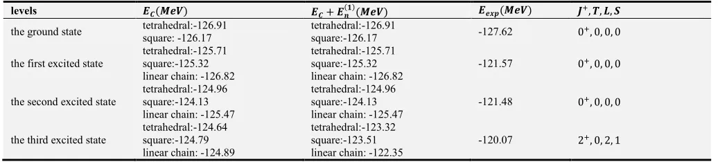
3745.44½ ¿ , respectively. Similar to the nucleus by fitting the ground state and the first excited state of the nucleus to the experimental data, we obtain the other parameters. Therefore, parameters of , , ! , and ! are equal 67MeV, 122.52MeV, 2fm, and 2.13fm, respectively[45-49]. Obtained results of Eq. (35) as . have been shown in Table (2) for the different structures that are the tetrahedral, square and linear chain. In this table, the value of ._f is calculated for every state by substituting Eq. (36) into Eq. (31). For example, ._f for the ground state, first excited state and the second excited state is equal to zero because these states are in the zero spin, but in the third excited state, it is not zero but it has different results for any of the three structures because these three structures have different wave functions. The value of ._f for the third excited state in the tetrahedral structure is equal to 1.32Mev. Also, ._f for this state in the structures of the square and linear chain are calculated as 1.28MeV and 2.54MeV, respectively. These results have been shown in the Table (2). From these two tables, one can see that the difference between the computational and experimental results for nucleus is less than . For example in the ground state, this difference for is equal to 1.24 MeV and for is equal to 0.71 MeV. Therefore, one can say that the cluster model

has better solutions for the nuclei with the number of more alpha particles. One of the other issues that will be obtained in this paper, is the configuration of the alpha particles for the nucleus in the different states. We consider three configurations for the first four states of this nucleus like the tetrahedral, square and linear chain that have different factors like strength of the Coulomb’s repulsion i.e. _", the wave function, the repulsive and attractive ranges of the central potential. The configuration of states of the nucleus is determined by comparing the obtained energy of each state to the experimental data. So, if the calculated energy for a state in a probable structure is nearer to the experimental data, then we consider the hypothetical structure as the actual configuration of that state. Therefore if the structure of the ground state of nucleus is square, so _" is equal to

4m4 + √2p = 31.185½ . ¡¾. By using this value for ", the energy level in Eq.(35) is equal to ( -126.17)MeV that it’s difference with the experimental data is more than the previous state, i.e. the tetrahedral structure that it’s level energy is -126.91MeV. This topic shows that the tetrahedral structure is the ground state form of nucleus (00). I.e, in the ground state of this nucleus, the distance of between of the alpha particles is equal.

Table 2. The energy levels of the nucleus .

the ground state tetrahedral:-126.91 square: -126.17

tetrahedral:-126.91

square:-126.17 -127.62 00, 0, 0, 0 the first excited state

tetrahedral:-125.71 square:-125.32 linear chain: -126.82

-121.57 00, 0, 0, 0

the second excited state

-121.48 00, 0, 0, 0

the third excited state

-120.07 20, 0, 2, 1

Now we will determine configuration of the first excited state of the nucleus [50]. If this structure is square, so " = 4m4 + √2p = 31.185½ . ¡¾ . Therefore the energy level of this state for the square structure according to Eq.(35) is equal -125.32MeV. Also, if the configuration of the first excited state is the linear chain, then _" is equal Á9

9 , i.e. " = 25.439½ . So the energy of the first excited state with the linear chain structure is equal to -126.82 MeV. Therefore to compare these results with the experimental data for the first excited state, i.e. the value of 121.57 MeV, somebody can conclude that the value of -125.32 MeV is nearer to the experimental data. So the configuration of the first excited state of the nucleus is square. Now, from Table (2) for the second excited state, one can simply understand that the energy of the square configuration is nearer to the experimental data. Therefore the configuration of the second excited state is square. Finally, for the third excited state, considering Table (2), the total energy of the linear chain structure equal to -122.35MeV is nearer to the experimental data. Therefore, the structure of the third excited state for nucleus in the cluster model is the

linear chain. This result is very important because it shows that in the higher excited states, the structure of this nucleus in the cluster model limit to the non-localized gas configuration, i.e. the decentralized structure. Of course, the structure of the ground state and the first excited state of this nucleus have been obtained already [38, 39].

4. Conclusions

(6)

comparing the calculated energy to the experimental data, we obtained that the ground state of the nucleus in the cluster model has the tetrahedral structure and configuration of the first and second excited state of this nucleus are as the square structure. Also, it was gotten that the third excited state of the nucleus in the cluster model has the linear chain structure which is a good result for this nucleus because this result show that the higher excited states of the nucleus in the cluster model limit to the non-localized gas configuration, i.e. the decentralized structure.

References

[1] G. Gamow, Proc. Roy. Soc. A, 126, 632 (1930).

[2] G. C. Hanna, alpha radioactivity, in E. Segre, (ed.), “Experimental Nuclear Physics”, vol. 3, John Wiley and Sons, Inc., New York, (1959).

[3] Y. Kanada-Enyo, Prog. Theor. Phys. 117, 655 (2007) [Erratum-ibid. 121, 895 (2009)].

[4] Y. Kanada-Enyo, Phys. Rev. Lett. 81, 5291 (1998).

[5] W. von Oertzen, M. Freer, and Y. Kanada-En’yo, “Nuclear clusters and nuclear molecules,” Phys. Rep., vol. 432, no. 2, pp. 43-113, (2006).

[6] H Yépez-Martínez et al, Phys. Rev. C 86, 034309 (2012). [7] H Yépez-Martínez et al, Phys. Rev. C 85, 014316 (2012). [8] P R Fraser et al, Phys. Rev. C 85, 014317 (2012). [9] Y Kanada-En’yo, Phys. Rev. C 89, 024302 (2014).

[10] Anjana Acharya, and Rajib Lochan Nayak, Int. J. Curr. Res, Vol. 8, pp. 27401-27406, (2016).

[11] Jinesh Kallunkathariyil, Zbigniew Sosin, and Andrzej Wieloch, Acta. Phys. Pol. B, 6, 1147-1150 (2013).

[12] J. A. Peacock, S. Cole, P. Norberg, C. M. Baugh, J. Bland-Hawthorn, T. Bridges, R. D. Cannon, M. Colless, C. Collins, and W. Couch, ”A measurement of the cosmological mass density from clustering in the 2dF Galaxy Redshift Survey,” Nature, vol. 410, no. 6825, pp. 169-173, (2001).

[13] M. Freer and A. C. Merchant, “Developments in the study of nuclear clustering in light even-even nuclei,” J. Phys. G Nucl. Part. Phys., vol. 23, no. 3, p. 261, (1997).

[14] M. Freer, “The clustered nucleus-cluster structures in stable and unstable nuclei,” Reports Prog. Phys., vol. 70, no. 12, p. 2149, (2007).

[15] M. Freer, “Clusters in nuclei,” Scholarpedia, vol. 5, no. 6, p. 9652, (2010).

[16] D. R. Tilley, H. R. Weller, and G. M. Hale, “Energy levels of light nuclei A= 4,” Nucl. Phys. A, vol. 541, no. 1, pp. 1-104, (1992). [17] G. Gamow, “Mass defect curve and nuclear constitution,”

Proc. R. Soc. London. Ser. A, Contain. Pap. a Math. Phys. Character, vol. 126, no. 803, pp. 632-644, (1930).

[18] K. Wildermuth and T. Kanellopoulos, “The ‘cluster model’ of the atomic nuclei,” Nucl. Phys., vol. 7, pp. 150-162, (1958).

[19] E. Rutherford, “The scattering of α and β particles by matter and the structure of the atom,” Philos. Mag., vol. 92, no. 4, pp. 379-398, (2012).

[20] Zbigniew Sosin, Jan Błocki, Jinesh Kallunkathariyil, Jerzy Łukasik and Piotr Pawłowski, arXiv:1506.06731 [nucl-th] (2016).

[21] L. R. Hafstad and E. Teller, Phys. Rev., vol. 54, no. 9, p.681, (1938).

[22] R Machleidt, Scholarpedia 9, 30710 (2014). [23] E Epelbaum et al, Rev. Mod. Phys. 81, 1773 (2009). [24] J S Hernandez et al, Phys. Rev. D 85, 071301 (2012). [25] E Z Liverts et al, Ann. Phys. 324, 388 (2009).

[26] K V Tretiakov et al, Phys. Status Solidi 251, 385 (2014). [27] J C Long et al, Nature 421, 922 (2003).

[28] S. Ali and A. R. Bodmer, Nucl. Phys., vol. 80, no. 1, pp. 99, (1966).

[29] Z. Papp, S. Moszkowski, Mod.Phys.Lett.B, vol. 22 pp. 2201, (2008).

[30] LR. Hafstad and E. Teller. Physical Review, 54:681, (1938). [31] D. Baye, P.-H. Heenen, Nucl. Phys. A 233, 304 (1974). [32] D. Baye, P.-H. Heenen, M. Liebert-Heinemann, Nucl. Phys. A

291, 230 (1977).

[33] D. Baye, P. Descouvement, in Proceedings of the fifth International Conference on Clustering aspects in nuclear and subnuclear systems, Kyoto, Japan, 25th July ed. by K. Ikeda, K. Katori, Y. Suzuki (1988), p. 103 [Supplement to the Journal of the Physical Society of Japan, vol. 58 (1989)].

[34] D. Baye, in Proceedings of the Sixth International Conference on Clusters in Nuclear Structure and Dynamics, Strasbourg, France, 6th September 1994, ed. by F. Haas (1994), p. 259. [35] A. F. Nikiforov and V. B. Uvarov, Special Functions of

Mathematical Physics (Birkhauser, Bassel, 1988).

[36] A. A. Rajabi and M. Hamzavi, Int. J. Theor. Phys. 7 (2013) 7. [37] Taiichi Yamada, Peter Schuck, Phys. Rev. C, 69, 024309

(2004).

[38] Bijker, Iachello, Evidence for Tetrahedral Symmetry in 16O. Phys. Rev. Lett. 112, 152501 (2014).

[39] E. Epelbaum, H. Krebs, T. A. Lahde, D. Lee, U. G. Meisner, and G. Rupak, Phys. Rev. Lett. 112, 102501 (2014).

[40] L. Liu and P. W. Zhao, Chin. Phys. C 36, 818 (2012). [41] T. Suhara et al., Phys. Rev. Lett. 112,062501 (2014). [42] M. R. Shojaei, et al., Mod. Phys. Lett. A, 23, 267, (2008). [43] M. R. Shojaei, et al., Inter. Jour. of Mod. Phys. E, 17, 6,

(2006).

[44] M. M. Giannini, et al., Nucl. Phys. A, 699, 308, (2002). [45] A. H. Al-Ghamdi, Awad A. Ibraheem, M. El-Azab Farid,

(7)

[46] M. A. Hassanain, Awad A. Ibraheem, and M. El-Azab Farid, Phys. Rev. C, 77, 034601 (2008).

[47] B. Buck, B. C. Dover, and J. P. Vary, Phys. Rev. C, 11,1803 (1975).

[48] B. Buck, H. Friedrich, and C. Wheatley, Nucl. Phys. A, 275, 246, (1977).

[49] M. N. A. Abdullah, S. Hossain, M. S. I. Sarker, S. K. Das, A.

S. B. Tariq, M. A. Uddin, A. K. Basak, S. Ali, H. M. Sen Gupta, and F. B. Malik, E. Phys. J. A, 18, 65, (2003);S. Hossain, M. N. A. Abdullah, K. M. Hasan, M. Asaduzzaman, M. A. R. Akanda, S. K. Das, A. S. B. Tariq, M. A. Uddin, A. K. Basak, S. Ali, and F. B. Malik, Phys. Lett. B, 636, 248, (2006).