IMPROVING PEAK-PICKING USING MULTIPLE TIME-STEP LOSS
FUNCTIONS
Carl Southall, Ryan Stables and Jason Hockman
DMT Lab, Birmingham City University, Birmingham, United Kingdom
{
carl.southall, ryan.stables, jason.hockman
}
@bcu.ac.uk
ABSTRACT
The majority of state-of-the-art methods for music infor-mation retrieval (MIR) tasks now utilise deep learning methods reliant on minimisation of loss functions such as cross entropy. For tasks that include framewise binary classification (e.g., onset detection, music transcription) classes are derived from output activation functions by identifying points of local maxima, or peaks. However, the operating principles behind peak picking are different to that of the cross entropy loss function, which minimises the absolute difference between the output and target values for a single frame. To generate activation functions more suited to peak-picking, we propose two versions of a new loss function that incorporates information from multiple time-steps: 1)multi-individual, which uses multiple indi-vidual time-step cross entropies; and 2) multi-difference, which directly compares the difference between sequential time-step outputs. We evaluate the newly proposed loss functions alongside standard cross entropy in the popular MIR tasks of onset detection and automatic drum tran-scription. The results highlight the effectiveness of these loss functions in the improvement of overall system ac-curacies for both MIR tasks. Additionally, directly com-paring the output from sequential time-steps in the multi-difference approach achieves the highest performance.
1. INTRODUCTION
At present, the state-of-the-art systems for many music in-formation retrieval (MIR) tasks utilise deep learning mod-els. Within the domain of dynamic time-series MIR tasks such as onset detection and music transcription, solutions are achieved through a binary classification of each time-stept. A binary classification output is typically limited to a range of [0,1] using a non-linear function (e.g., sigmoid, softmax). For classification purposes the output is subse-quently rounded to either 0or1. However, in framewise binary classification tasks using this approach has proven to be less effective [7]. In the example presented in Fig-ure 1, a framewise output activation functiony˜is shown in
c
Carl Southall, Ryan Stables and Jason Hockman. Li-censed under a Creative Commons Attribution 4.0 International License (CC BY 4.0).Attribution: Carl Southall, Ryan Stables and Jason Hock-man. “Improving Peak-picking Using Multiple Time-step Loss Func-tions”, 19th International Society for Music Information Retrieval Con-ference, Paris, France, 2018.
Figure 1. A true positive is missed using the rounding approach, but is successfully selected through peak picking (circled point). The solid line denotes the output, the dotted line the target, the dashed line the 0.5 rounding threshold and the dash-dotted line the peak-picking threshold.
which the values ideally associated with a class label (i.e., value) of1do not exceed0.5. Whiley˜clearly shows the presence of an event as apeak, it would be identified as a false negative (y˜t<0.5).
1.1 Peak Picking
To overcome the problem posed in Figure 1, the majority of framewise binary classification systems utilise peak pick-ing, which differentiates between classes by identifying lo-cal maxima. Multiple peak-picking approaches have been proposed in the literature [1, 4, 12, 16] and follow a general process as shown in Figure 1. Here, a point is selected as a peak if it is the maximum value within a local window and above a thresholdτ. In [16] the threshold is determined by calculating the mean of a window, controlled usingδ, a user determined constantλand maximum and minimum values (tmaxandtmin).
τt=mean(˜yt−δ: ˜yt+δ)∗λ (1)
τt=
tmax, τ > tmax
An onset classification vectorOis achieved by determin-ing if each time-step ofy˜is the maximum value within the surrounding number of frames, set usingΩ, and above the thresholdτ:
Ot=
1, y˜t==max(˜yt−Ω: ˜yt+Ω) & y˜t> τt
0, otherwise.
(3)
1.2 Loss Functions
The overall loss (often referred to as thecost)Lrepresents the error of a system within a single value. It is calculated by comparing the difference between the desired ground truth y and the actual outputy˜[10]. Within audio based time-step classification tasks it is calculated by taking the mean of the individual time-step losseslt:
L= 1
T
T
X
t=1
lt. (4)
Lis a component of back propagation (and truncated back propagation) which is used to calculate the gradients G
used in updating the trainable parameters of the model Θ
with learning rateµ.
Θ←Θ−µ· G (5)
Commonly used loss functions for calculating lt include mean squared error (MS) (eq. 6) and cross entropy (CE) (eq. 7) [5].
lmst {yt,y˜t}= (yt−y˜t)2 (6)
ltce{yt,y˜t}=ytlog (˜yt) + (1−yt) log (1−y˜t) (7)
Both of these loss functions are suited to differentiating between binary classes using rounding as they aim to min-imise the absolute difference between the targets y and the output y. In the majority of MIR tasks˜ CEis more suited thanMSdue to its greater penalization of large er-rors [14, 16, 22].
1.3 Motivation
In the peak-picking process, multiple frames are utilized in both the calculation of a threshold as well as the peak selection. However, in theMSandCEcalculations only the current time-steptis used in measuring the difference be-tween the target y and outputy. In order for the loss to˜
reflect peak salience (i.e., the clarity of the local maxima) and to ensure that the output activation function is suit-able for peak-picking, then multiple time-steps should be included within the loss function calculation. To this end, we propose two versions of a new loss function which not only measures the absolute difference betweenyandy, but˜
also allows for peak salience to be maintained. We then evaluate the worth of these functions within the tasks of onset detection and automatic drum transcription (ADT).
The remainder of this paper is structured as follows: Section 2 presents the proposed loss functions and Section
3 gives an overview of the evaluation. The results and dis-cussion are presented in Section 4 and the conclusions and future work are presented in Section 5.
2. METHOD
For a loss function to represent an understanding of peak salience, it must include at least three points:y˜t−1: ˜yt+1.
We propose combining CE and a peak salience measure into a single loss function termed peakiness cross entropy (PCE):
lpcet = 1 2 γl
t ce{y
t,y˜t
}+ (1−γ)(ltp+ltf)
, (8)
where the first part of the equation is the standard cross entropy (CE) of the current time-stept. The second part of the function is a peak salience measure that consists of two variables:lp, which focuses on the previous time-step
andlf, which focuses on the future (t+ 1) time step.γis
used to control the weighting between standardCEand the peakiness measure. We propose two methods for achieving lpandlf: a combination of multiple individual time-step
calculations and a direct comparison of the differences be-tween multiple time-steps.
2.1 Multi-individual
The multi-individual (MI) method calculates lp andlf as
individual time step cross entropies of previous and future time-steps:
ltp=lcet {yt−1,y˜t−1} (9)
ltf =ltce{yt+1,y˜t+1}. (10)
This ensures that updates toy˜tdo not cause greater nega-tive updates toy˜t−1andy˜t+1.
2.2 Multi-difference
AlthoughMIutilizes multiple time-steps it does not com-pare absolute differences between sequential time-steps. To achieve this, we propose an additional calculation of lp andlf, termed multi-difference (MD), which measures
the absolute differences between sequential time-steps of the targetyand the outputy. The first version of˜ MD(MMD), utilizesMS. The second version (WMD) utilizes an updated version of theCEequation, termed weighted cross entropy (WCE):
ltwce{yt,y˜t}= (1−φ)ytlog (˜yt) +φ(1−yt) log (1−y˜t), (11) which allows the strength of each half of the equation to be controlled using the weighting parameter φ. The first half of theWCEequation (henceforth referred to asWCE-FN) aims to reduce false negatives by producing a loss value proportional to the difference between sequential time-steps ofytandy˜t. The second half of the WCEequation
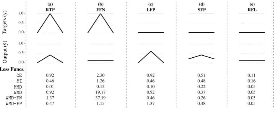
Figure 2. Example activation function scenarios with corresponding loss values output from each loss function. From left to right: a raised true positive (RTP), a flat line false negative (FFN), a large false positive (LFP), a small raised false positive (SFP) and a raised flat line (RFL).
as it outputs a larger value if there is a large undesirable difference between sequential frames.lt
pandlft inMMDand
WMDare calculated respectively using:
ltp=
ltwce{|yt−yt−1|,|y˜t−y˜t−1|}, W M D,
ltms{|yt−yt−1|,|y˜t−y˜t−1|}, M M D, (12)
ltf =
lt
wce{|yt−yt+1|,|y˜t−y˜t+1|}, W M D,
lt
ms{|yt−yt+1|,|y˜t−y˜t+1|}, M M D.
(13) Truncated back propagation is used to calculate the gradi-ents for all loss functions. The presented implementation utilises the automatic differentiation functions built into the Tensorflow1 library for this purpose.
2.3 Example Loss Function Scenarios
Figure 2 presents five example activation function sce-narios. The loss values achieved by CE, MI, MMD, WMD
and the two separated halves of WMD: WMD-FN (φ = 0) andWMD-FP (φ = 1), are presented withγ = 0.5. The targets are presented at the top and the output activation function on the bottom. It is worth noting that all of the loss functions that utilize CE can be directly com-pared but MMD is relative to itself (i.e., the MMD values might seem small relative to the other loss values but not relative to other values of MMD). If all frames of the output are correct then all of the loss functions output zero.
(a) Reduced true positive: The first example shows
a reduced true positive where the surrounding frames are correct. In this caseCEandWMDoutput the largest values as this peak could fall below the peak-picking threshold.
1https://www.tensorflow.org
(b) Flat line false negative: The second example
shows a false negative where the output is a flat line. In this case high relative error values are given by all of the loss functions, however larger error values are given by MMD and especially the FN suppression half of WMD. This example would generally not be selected during peak-picking.
(c) Large false positive: The third example shows a
false positive where the surrounding frames are correct. In this case high values are given by CE, MMD and the false positive suppression part ofWMD, as this would be an incorrectly selected peak.
(d) Small raised false positive: The fourth example
again shows a false positive, similar to the previous example, but the surrounding frames are raised resulting in a less salient false positive. In this case lower values are given byMIandWMD-FP, thanCE, as this peak is not as salient as the one in example three (i.e., large false positive).
(e) Raised flat line: The final example presents a
raised flat line. In this case theMMDandWMDloss functions penalize less than CE andMI. While the absolute values are slightly wrong, the difference between the sequential frames is correct, resulting in no peaks being correctly chosen.
3. EVALUATION
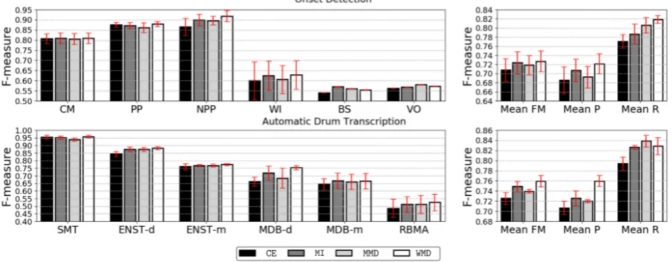
Figure 3. Subset mean system F-measure results for the four implemented cost functions for onset detection and automatic drum transcription. The individual subset F-measure results are on the left and the mean subset F-measure, precision and recall results are on the right. The red error plots display the standard deviations across the folds.
based models which have achieved state-of-the-art results for both of the tasks in recent years. Standard F-measure, derived from precision and recall, is used as the evalua-tion metric with onset candidates being accepted if they fall within30ms of the ground truth annotations (i.e., win-dow of acceptance). If onset candidates fall within 30ms of each other, they are combined into a single onset at the middle location (i.e., window of combination).
3.1 Onset Detection (OD)
For the OD evaluation, we utilize the same datasets and subset splits as used in [3], consisting of: complex mix-tures (CM), pitched percussion (PP), non-pitched percus-sion (NPP), wind instruments (WI), bowed strings (BS) and vocals (VO). As OD is a binary classification task, all systems are implemented with a two neuron softmax out-put layer, one neuron corresponds to an onset and the other neuron corresponds to the absence of an onset.
3.2 Automatic Drum Transcription (ADT)
For the ADT evaluation, we utilize four ADT datasets: IDMT-SMT-Drums [6], ENST-Drums minus one subset [8], MDB-Drums [18] and RBMA-2013 [21]. To observe trends between contexts, the datasets are divided into the three groups proposed in [23]: 1) drum only (DTD) con-sisting of IDMT-SMT-Drums, 2) drums in the presence of extra percussion (DTP) consisting of the drum-only ver-sions ENST-d and MDB-d and 3) drums in the presence of extra percussion and melodic instruments (DTM), which consist of the polyphonic versions ENST-m, MDB-m and RBMA-2013. ENST-m is created by combining the ENST drum tracks and the accompaniment files using ratios of 23 and 13 respectively, as done in [6, 9, 15, 20, 24]. A three-neuron sigmoid output layer is used for all implemented ADT systems, with the neurons corresponding to the three observed drum instruments (i.e., KD, SD and HH).
3.3 Systems
Four different neural network based systems are imple-mented. All systems consist of the same overlying struc-ture: First, input features are fed into a pre-trained neural network model. Peak-picking is then performed to deter-mine the locations of the onset candidates using the algo-rithm from [16] (eq.1:3).
3.3.1 Input Features
For both tasks we use the same framewise logarithmic spectral input features x generated using the madmom Python library [2]. The input audio (16-bit .wav file sam-pled at 44.1 kHz) is segmented intoT frames using a Han-ning window of msamples (m = 2048) with a m2 hop-size. A logarithmic frequency representation of each of the frames is created using a similar process to [22]. The mag-nitudes of a discrete Fourier are transformed into a loga-rithmic scale (20Hz–20kHz) using twelve triangular filters per octave. This results in a 84 xT logarithmic spectro-gram.
3.3.2 lstmpB
The lstmpB system is based on the system presented in [23] and the baseline system used in [16]. It consists of two 50-neuron hidden layers containing long short-term mem-ory cells with peephole connections. The input features are processed in a framewise manner.
3.3.3 lstmpSA3B
Figure 4. Individual system mean subset F-measure re-sults for the proposed cost functions in OD and ADT tasks. Red bars denote standard deviations across folds.
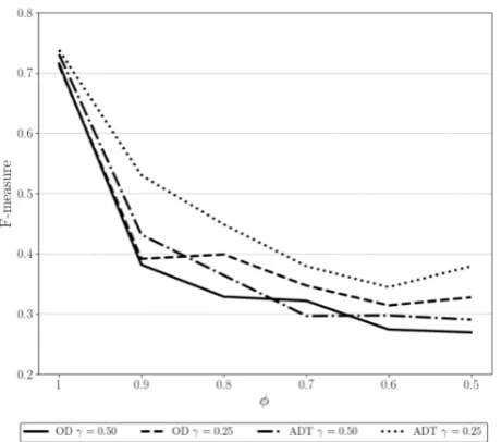
Figure 5. Mean system and mean subset results for differ-ent values ofWMDparameters (γandφ) in onset detection (OD) and automatic drum transcription (ADT) evaluations.
3.3.4 lstmpSA3B-F5
ThelstmpSA3B-F5 system is identical to thelstmpSA3B
system with a larger number of input features used. A total of 11 frames (5 either side of the current frame (xt−5 :
xt+5)) are used for each time-step.
3.3.5 cnnSA3B-F5
ThecnnSA3B-F5 [17] combines the convolutional recur-rent neural network proposed in [22] and the soft atten-tion mechanism proposed in [16]. It contains two convo-lutional layers consisting of 3x3 filters, 3x3 max pooling, dropouts [19] and batch normalization [11], with the first layer consisting of 32 channels and the second 64 chan-nels. It contains the same soft attention mechanism output
layer and the same input feature size aslstmpSA3B-F5.
3.3.6 Training
All systems are trained using mini-batch gradient descent with the Adam optimizer [13]. An initial learning rate of 0.003 is used and three-fold cross validation is per-formed. Each mini-batch consists of 10 randomly chosen, 100 time-step segments and the data is divided by track into 70% training, 15% validation and 15% testing sets. The training data is used to optimize the systems and the validation data is used to prevent overfitting and to opti-mize the peak-picking parameters. For datasets contain-ing subsets (i.e., IDMT-SMT Drums and ENST Drums) the splits are performed evenly across the subsets.
4. RESULTS AND DISCUSSION
4.1 Subset Performance
Figure 3 presents the subset results for all cost functions in both evaluations. The red error bars represent standard de-viation across folds. The OD results are derived from the mean of the systems and the ADT results are derived from the mean of the systems and the mean of the observed drum instruments (i.e., KD, SD and HH). The left part of the fig-ure presents the individual subset F-measfig-ures and the right part of the figure presents the mean subset F-measure, pre-cision and recall. In both MIR tasks, all three of the newly proposed cost functions achieved a higher mean subset F-measure than standardCE, withWMDperforming the best in both. Within the ADT evaluation a higher performance is achieved for all three observed drum instruments. A slightly larger increase in performance was witnessed in the ADT task and both versions of the MDcost function achieve higher mean subset F-measures thanMI. This high-lights that measuring the absolute differences between se-quential frames does improve performance. The mean sub-set precision and recall results highlight that in all cases the newly proposed cost functions achieve higher precision and recall scores than standardCE. In the OD evaluation the highest increase in performance betweenWMDandCEis in the NPP subset. In the ADT evaluation the largest increase is seen within the DTP subsets (ENST-d and MDB-d). For all subsets in both evaluations the highest F-measure is achieved by one of the three newly proposed cost functions and the error bars show that this improvement occurs in all of the folds. Results from t-tests highlight that theWMD sys-tems improvement overCEwithin the BS and mean recall OD categories and MDB-d, mean F-measure and precision ADT categories are significant (ρ <0.05).
4.2 Individual System Performance
improve performance and that this increase is not just as-sociated with one system. The highest F-measure and the largest increase relative to CE is achieved by the
cnnSA3B-F5 system using theWMDcost function.
4.3 WMD Parameters
Figure 5 presents the mean system, mean subset F-measure results for different parameter settings of theWMDcost func-tion. Plots of sixφvalues forγ = 0.25andγ = 0.5are presented for both evaluations. For anyφvalues less than one, there is a dramatic decrease in performance which suggests that the false negative suppression half of theWCE
function has a negative effect on performance. This is pos-sibly due to the extremely high value given to flat parts of the activation function (see Figure 2), causing these parts of the activation function to become noisy. This suggests that the improvement is due to the false positive suppres-sion half of theWMDsystem. As this alone achieves higher F-measures than the other proposed cost functions, then it also suggests that their improvement is also due to the suppression of false positives. However, the false nega-tive suppression in those cost functions do not cause reper-cussions. Asγ(i.e., weighting of peak salience measure) increases (0.5 = even weighting with standard CE) then the performance decreases. This trend continues with all values below 0.5 and with the other two proposed loss functions. The highest F-measures were achieved with γ=0.25 (StandardCEis weighted twice as much as the peak salience measure) for all three proposed loss functions. To categorically identify ideal parameter settings for a partic-ular scenario, a grid search would be required. However, the results suggest thatγ= 0.25andφ= 1would always be optimal.
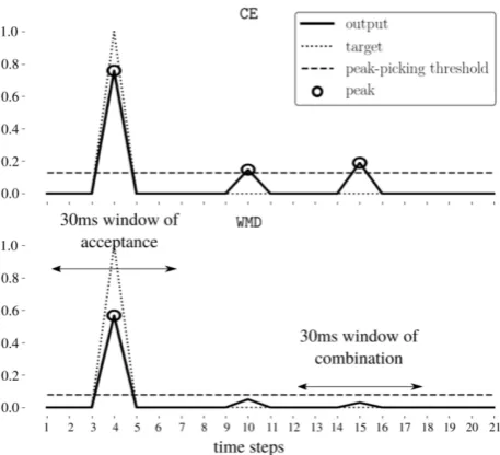
4.4 Understanding the Improvement
After visual comparison of the output activation functions a common situation in which the newly proposed loss func-tions achieve higher performance was observed. Figure 6 presents an example of this situation, with the top diagram showing the output activation function using CE and the bottom diagram showing the activation function when us-ing the highest performus-ing version ofWMD. In theCE dia-gram, there are two spikes to the right that are wrongly de-tected as peaks but in theWMDversion these peaks are less salient, resulting in no false positives. The consequence of this is that the actual true positive within in the WMD ver-sion has a lower amplitude than the one in theCEversion. However, this has no effect on performance as the true pos-itive is still a clear peak and correctly chosen within both
CEandWMDversions. We believe this situation occurs be-cause withinCEa higher error is given to the true positive than the combination of the two smaller false positive er-rors. This causes the true positive to be closer to the tar-gety but consequentially causes the false positive spikes. Within theWMDversion, the false positive suppression as-signs a greater loss value to the two false positive spikes than the reduced true positive, ensuring that the spikes are
Figure 6. Example ofWMDloss function reducing the num-ber of false positives by suppressing false spikes.CEoutput activation function (top) andWMDoutput activation function (bottom) with outputy˜(solid lines), targety(dotted lines) and the peak-picking threshold (dashed lines). Circles de-note selected peaks and arrowed lines show windows of acceptance and combination.
not selected by the peak-picking algorithm. This reduc-tion of noise in the activareduc-tion funcreduc-tion results in less false positives but also enables the peak-picking threshold to be lower, enabling more true positives to be selected. This effect could likely explain both the increase in recall and precision.
5. CONCLUSIONS AND FUTURE WORK
We have developed three new loss functions in an at-tempt to generate activation functions more suited to peak-picking. The new loss functions utilise information from multiple time-steps which allow them to measure both the absolute values and to maintain peak salience by compar-ing sequential time-steps. We evaluated the newly pro-posed loss functions against standardCEusing four neural network-based systems in the MIR tasks of onset detection and ADT. The results highlight that all three of the newly proposed cost functions do improve performance, with the
WMD loss function achieving the highest accuracy. This work focuses on the inclusion of a single frame on either side of the current time-step. Future work could explore the potential benefit of using a greater number of frames and a version of theWMDequation in which the false nega-tive suppression component does not neganega-tively influence the outcome. Additionally, to make the system end-to-end, the evaluation methodology (i.e., F-measure and tolerance windows) could also be incorporated within the loss tions. Open source implementations of the new loss func-tions are available online.2
2https://github.com/CarlSouthall/PP_loss_
6. REFERENCES
[1] Juan Pablo Bello, Laurent Daudet, Samer Abdallah, Chris Duxbury, Mike Davies, and Mark B. Sandler. A tutorial on onset detection in music signals. IEEE Transactions on Audio, Speech, and Language Pro-cessing, 13(5):1–13, 2005.
[2] Sebastian B¨ock, Filip Korzeniowski, Jan Schl¨uter, Flo-rian Krebs, and Gerhard Widmer. madmom: A new Python audio and music signal processing library. In Proceedings of the ACM International Conference on Multimedia, pages 1174–1178, Amsterdam, The Netherlands, 2016.
[3] Sebastian B¨ock, Florian Krebs, and Markus Schedl. Evaluating the online capabilities of onset detection methods. InProceedings of the 13th International So-ciety for Music Information Retrieval Conference (IS-MIR), Porto, Portugal, 2012.
[4] Sebastian B¨ock, Jan Schl¨uter, and Gerhard Widmer. Enhanced peak picking for onset detection with recur-rent neural networks. InProceedings of the 6th Inter-national Workshop on Machine Learning and Music (MML), pages 15–18, Prague, Czech Republic, 2013.
[5] Pieter-Tjerk de Boer, Dirk Kroese, Shie Mannor, and Reuven Y. Rubinstein. A tutorial on the cross-entropy method.Annals of operations research, 134(1):19–67, 1 2005.
[6] Christian Dittmar and Daniel G¨artner. Real-time tran-scription and separation of drum recordings based on NMF decomposition. In Proceedings of the Interna-tional Conference on Digital Audio Effects (DAFx), pages 187–194, Erlangen, Germany, 2014.
[7] Florian Eyben, Sebastian B¨ock, Bj¨orn Schuller, and Alex Graves. Universal onset detection with bidirec-tional long-short term memory neural networks. In
Proceedings of the 11th International Society for Mu-sic Information Retrieval Conference (ISMIR), pages 589–594, Utrecht, The Netherlands, 2010.
[8] Olivier Gillet and Ga¨el Richard. Enst-drums: an exten-sive audio-visual database for drum signals processing. InProceedings of the 7th International Society for Mu-sic Information Retrieval Conference (ISMIR), pages 156–159, Victoria, Canada, 2006.
[9] Olivier Gillet and Ga¨el Richard. Transcription and sep-aration of drum signals from polyphonic music.IEEE Transactions on Audio, Speech, and Language Pro-cessing, 16(3):529–540, 2008.
[10] Ian Goodfellow, Yoshua Bengio, and Aaron Courville.
Deep Learning. MIT Press, 2016.
[11] Sergey Ioffe and Christian Szegedy. Batch normaliza-tion: Accelerating deep network training by reducing internal covariate shift. InInternational Conference on Machine Learning, pages 448–456, 2015.
[12] Ismo Kauppinen. Methods for detecting impulsive noise in speech and audio signals,. In Proceedings of the 14th International Conference on Digital Sig-nal Processing (DSP2002), pages 967–970, Santorini, Greece, 2002.
[13] Diederik P. Kingma and Jimmy Ba. Adam: A method for stochastic optimization. CoRR, abs/1412.6980, 2014.
[14] Jan Schluter and Sebastian Bock. Improved musical onset detection with convolutional neural networks. In Proceedings of the 2014 IEEE International Con-ference on Acoustics, Speech and Signal Processing (ICASSP), pages 6979–6983, 2014.
[15] Carl Southall, Ryan Stables, and Jason Hockman. Au-tomatic drum transcription using bi-directional recur-rent neural networks. In Proceedings of the 17th In-ternational Society for Music Information Retrieval Conference (ISMIR), pages 591–597, New York City, United States, 2016.
[16] Carl Southall, Ryan Stables, and Jason Hockman. Automatic drum transcription for polyphonic record-ings using soft attention mechanisms and convolutional neural networks. InProceedings of the 18th Interna-tional Society for Music Information Retrieval Confer-ence (ISMIR), pages 606–612, Suzhou, China, 2017.
[17] Carl Southall, Ryan Stables, and Jason Hockman. Player vs transcriber: A game approach to data manip-ulation for automatic drum transcription. In Proceed-ings of the 19th International Society for Music Infor-mation Retrieval Conference (ISMIR), Paris, France, 2018.
[18] Carl Southall, Chih-Wei Wu, Alexander Lerch, and Jason Hockman. MDB drums an annotated subset of medleyDB for automatic drum transcription. In Pro-ceedings of the 18th International Society for Music Information Retrieval Conference (ISMIR), Suzhou, China, 2017.
[19] Nitish Srivastava, Geoffrey Hinton, Alex Krizhevsky, Ilya Sutskever, and Ruslan Salakhutdinov. Dropout: A simple way to prevent neural networks from overfitting. Journal of Machine Learning Research, 15(1):1929–1958, 2014.
[20] Richard Vogl, Matthias Dorfer, and Peter Knees. Re-current neural networks for drum transcription. In Pro-ceedings of the 17th International Society for Music Information Retrieval Conference (ISMIR), pages 730– 736, New York City, United States, 2016.
[22] Richard Vogl, Matthias Dorfer, Gerhard Widmer, and Peter Knees. Drum transcription via joint beat and drum modeling using convolutional recurrent neural networks. InProceedings of the 18th International So-ciety for Music Information Retrieval Conference (IS-MIR), pages 150–157, Suzhou, China, 2017.
[23] Chih-Wei Wu, Christian Dittmar, Carl Southall, Richard Vogl, Gerhard Widmer, Jason Hockman, Meinard M¨uller, and Alexander Lerch. A Review of Automatic Drum Transcription. IEEE/ACM Transac-tions on Audio, Speech, and Language Processing, 26(9):1457–1483, 2018.