DOI 10.1186/s13408-015-0026-5
R E S E A R C H Open Access
Conditions for Multi-functionality in a Rhythm
Generating Network Inspired by Turtle Scratching
Abigail C. Snyder1·Jonathan E. Rubin1
Received: 27 January 2015 / Accepted: 2 June 2015 /
© 2015 Snyder and Rubin. This article is distributed under the terms of the Creative Commons Attribution 4.0 International License (http://creativecommons.org/licenses/by/4.0/), which permits unrestricted use, distribution, and reproduction in any medium, provided you give appropriate credit to the original author(s) and the source, provide a link to the Creative Commons license, and indicate if changes were made.
Abstract Rhythmic behaviors such as breathing, walking, and scratching are vital
to many species. Such behaviors can emerge from groups of neurons, called central pattern generators, in the absence of rhythmic inputs. In vertebrates, the identifica-tion of the cells that constitute the central pattern generator for particular rhythmic behaviors is difficult, and often, its existence has only been inferred. For example, under experimental conditions, intact turtles generate several rhythmic scratch motor patterns corresponding to non-rhythmic stimulation of different body regions. These patterns feature alternating phases of motoneuron activation that occur repeatedly, with different patterns distinguished by the relative timing and duration of activity of hip extensor, hip flexor, and knee extensor motoneurons. While the central pattern generator network responsible for these outputs has not been located, there is hope to use motoneuron recordings to deduce its properties. To this end, this work presents a model of a previously proposed central pattern generator network and analyzes its capability to produce two distinct scratch rhythms from a single neuron pool, se-lected by different combinations of tonic drive parameters but with fixed strengths of connections within the network. We show through simulation that the proposed network can achieve the desired multi-functionality, even though it relies on hip unit generators to recruit appropriately timed knee extensor motoneuron activity, includ-ing a delay relative to hip activation in rostral scratch. Furthermore, we develop a phase space representation, focusing on the inputs to and the intrinsic slow variable of the knee extensor motoneuron, which we use to derive sufficient conditions for the network to realize each rhythm and which illustrates the role of a saddle-node bifurcation in achieving the knee extensor delay. This framework is harnessed to
con-B
A.C. Snyder [email protected]J.E. Rubin [email protected]
1 Department of Mathematics, University of Pittsburgh, 301 Thackeray Hall, Pittsburgh, PA
sider bistability and to make predictions about the responses of the scratch rhythms to input changes for future experimental testing.
Keywords Central pattern generator·Turtle motor rhythms·Phase plane analysis· Slow dynamics
1 Introduction
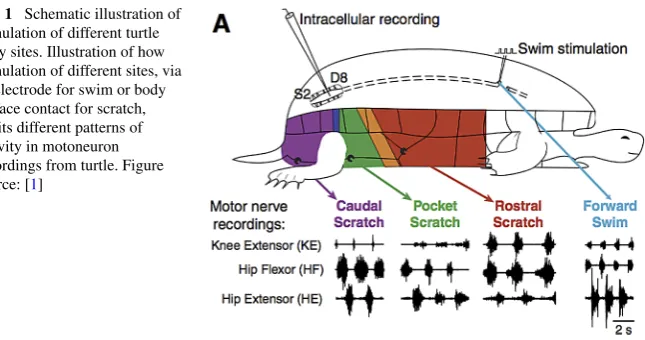
Under experimental conditions, intact turtles are observed to generate a variety of rhythmic motor patterns corresponding to stimulation of different body regions (in-cluding caudal scratch, rostral scratch, pocket scratch, and forward swim; see Fig.1) [1]. All of these patterns feature alternating phases of motoneuron activation that oc-cur repeatedly, while different patterns are distinguished by the relative timing and duration of activity of hip extensor motoneurons, hip flexor motoneurons and knee extensor motoneurons. Notably, these stable, rhythmic behaviors arise in the absence of rhythmic stimulation, suggesting that a central pattern generator (CPG) may be re-sponsible. Spinalized turtles, in which motor pathways from higher brain areas have been cut, display corresponding fictive behaviors in response to the same forms of stimulation, which suggests that necessary components for rhythm generation are present in the brain stem and spinal cord [1–4]. However, even with restriction to these areas, the complexity of the neuronal networks in turtle have made it impracti-cal to locate the relevant CPG neurons experimentally.
As an alternative, researchers have, on theoretical grounds, proposed structures that may represent important components or principles involved in the function of the relevant CPGs [5–9]. Computational methods offer a natural means to investigate these structures’ properties and generate predictions about them that may guide future experimental investigations. In this work, we use computational methods to study a model CPG network that was previously suggested as a kernel for turtle pocket scratch (pocket) and rostral scratch (rostral) motor pattern generation [4]. Specifi-cally, we demonstrate that a simulated version of this model can generate both of these rhythms, selected only by the relative levels of certain constant inputs, for fixed parameter values, and we derive conditions on model parameters that ensure that this dual functionality will exist.
Fig. 1 Schematic illustration of
stimulation of different turtle body sites. Illustration of how stimulation of different sites, via an electrode for swim or body surface contact for scratch, elicits different patterns of activity in motoneuron recordings from turtle. Figure source: [1]
of projection targets and instead show that by considering only hip-related pools of excitatory and inhibitory interneurons, each projecting to both hip and knee MNs, appropriate knee-hip timing relations can be produced.
This result may seem surprising in light of past theory; however, a variety of ex-perimental works [2–4,12] have shown that knee extensor MNs receive temporally overlapping excitation and inhibition and that the time courses of the inputs to knee extensor MNs are similar to those of inputs to hip flexor MNs in rostral and to hip extensor MNs in pocket. Berkowitz and Stein argued that an architecture featuring excitatory and inhibitory pools of interneurons for each of hip extensor and hip flexor (with each MN population active in synchrony with its respective excitatory pool), which also project to knee extensor MNs, could be more consistent with experimen-tal findings than other architectures [4]. The idea that different rhythm generators can control knee extensor MN timing in different rhythms also fits in with recent obser-vations from experiments in the mouse hindlimb locomotor network, which suggest that intrinsically rhythmic interneuron modules can be flexibly recruited to drive MN pools [13]. Certainly, knee flexor motoneurons are also involved in the generation of these rhythms [9,14,15]. Hip extension, hip flexion, and knee extension are sufficient to typify the rhythms, however, and previous studies have focused on these three MN populations [1–4], so we do not consider hip flexor activity in this work.
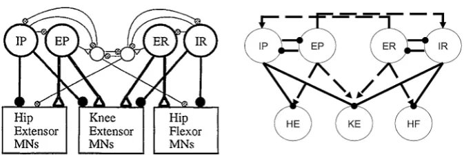
Fig. 2 Proposed (left) and implemented (right) network architectures. Solid circles correspond to
in-hibitory synaptic connections, open triangles (left) and dashed arrows (right) to excitatory ones. Figure source for proposed architecture: [4]
The remainder of this paper is organized as follows. In Sect.2, we present the details of the implemented architecture and the specific mathematical choices made to model it. Section3has three main parts. First, we show results of simulations that illustrate the multi-functionality of the model network (Sect.3.1). Next, we derive a reduced slow phase space based on knee extensor motoneuron dynamics in which analysis becomes tractable and apply this framework to elucidate the fundamental mechanisms that generate the network dynamics we observe (Sect.3.2). Finally, we harness the phase space to consider additional experimental findings and new pre-dictions relating to bistability and to responses to changes in inputs (Sect.3.3). The paper concludes with a discussion (Sect.4).
2 Model
A possible motor CPG architecture, differing from the traditional unit pattern gener-ator (UPG) framework with a separate interneuron pool driving each muscle’s mo-toneurons [11,16], was proposed based on experimental results on turtle scratching rhythms [4] (Fig.2, left). As has been well established, however, drawing a plausi-ble wiring diagram for a rhythmic circuit does not allow the immediate inference of actual circuit activity patterns [17]. To explore network dynamics, we implement a simplified version of the proposed architecture, featuring a layer of interneuron pools indexed by labelsi∈ {IP,EP,ER,IR}interacting with each other and feeding for-ward to a layer of MNs indexed by labelsi∈ {HE,KE,HF}that do not interact. In lieu of an excitatory pool exciting an inhibitory sub-population that in turn inhibits or disinhibits inhibitory pools as originally proposed (e.g. EP excites a sub-population that inhibits IP and disinhibits IR, Fig.2, left), in our model E and I pools are linked, for simplicity, via direct synaptic connections (Fig.2, right). A variety of notation associated with this model and its dynamics will be introduced throughout the paper, which we summarize in Table1.
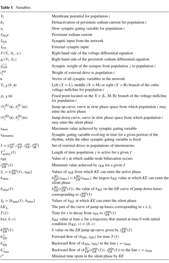
Table 1 Variables
Vi Membrane potential for populationi
hi Deinactivation of persistent sodium current for populationi si Slow synaptic gating variable for populationi
INaP Persistent sodium current Isyn Synaptic input from the network Iext External synaptic input
F (Vi, hi, si) Right hand side of the voltage differential equation
gi(Vi, hi) Right hand side of the persistent sodium differential equation gsyni,j Synaptic weight of the synapse from populationjto populationi iexti Weight of external drive to populationi
s Vector of all synaptic variables in the network
Vi,X(h,s) Left (X=L), middle (X=M) or right (X=R) branch of the cubic
voltage nullcline for populationi
pi,X(s) Fixed point located on theX∈ {L,M,R}branch of the voltage nullcline
for populationi
(ViJU(s), hJUi (s)) Jump up curve, curve in slow phase space from which populationimay enter the active phase
(ViJD(s), hJDi (s)) Jump down curve, curve in slow phase space from which populationi
may enter the silent phase
smax Maximum value achieved by synaptic gating variable
sdynamic Synaptic gating variable evolving in time for a given portion of the
rhythm, while the other synaptic gating variable is fixed
I= {iextIP, iextEP, iextER, iextIR} Set of external drives to populations of interneurons
Tactivej (I ) Length of time populationjis active for a givenI sSN Value ofsat which saddle-node bifurcation occurs sminER(I ) Minimum value achieved bysERfor a givenI
Is= [sERmin(I ), sSN] Values ofsERfrom which KE can enter the active phase
hmax hJDEP(smax)=hJDER(smax), the largesthKEvalue at which KE can enter the
silent phase
hmin(I ) hJDER(sminER(I )), the value ofhKEon the ER curve of jump down knees
corresponding tosERmin(I )
Ih= [hmin(I ), hmax] Values ofhKEat which KE can enter the silent phase
LKIs The part of the curve of jump up knees corresponding tos∈Is T (I ) Time forsto decay fromsSNtosminER(I )
h(a;b, c) hKEvalue at timeafor a trajectory that started at time 0 with initial
condition(hKE, s)=(b, c)
hminER(I ) hvalue on the ER jump up curve given bysminER(I ) h+SN Forward flow of(hSN, sSN)for timeT (I ) h−SN Backward flow of(hSN, sSN)to the lines=smax h−smin Backward flow of(h
JU
ER(sERmin(I )), sminER(I ))to the lines=smax
interneuron population IP, while HF activates in synchrony with its excitatory in-terneuron population ER, which activates in antiphase with the inhibitory inin-terneuron population IR. The nature of the rhythms (Fig.1) indicates additionally that HE and HF must activate in antiphase for both rhythms, with HF activated longer in rostral and HE activated longer in pocket. It was hypothesized that KE receives inputs that are similar to those received by HF in rostral and similar to those received by HE in pocket [3]. The subsequently proposed architecture in Fig.2, however, suggests that the inputs to KE are proportional to those to both HE and HF, which makes it less clear why KE synchronizes with HF, after some delay, in rostral and with HE in pocket (Fig.1), which is what we seek to explain.
Since we seek to assess the basic rhythm generating capabilities of the proposed architecture, we model each neuronal population in the network as a single cell, leav-ing issues of heterogeneity for future investigation; we nonetheless refer to each as a “population” in the remainder of the paper (cf. [6]). Inasmuch as the relevant rhythm generating neurons in turtle have not been identified, the specific currents that are central to their rhythmicity are not known. Given this situation, it makes sense to avoid overly specific assumptions about the dynamics of model components. The dy-namically simple Wilson–Cowan equations were used in related previous work [5] to model forward swim and caudal scratch rhythms. However, there is a delay in the onset of knee extensor activity relative to hip extensor in caudal scratch that was not modeled in the earlier study. Since the delay of knee extensor onset in rostral scratch is one of the key features that we seek to model, and phase plane considerations sug-gest that the monotone nullclines of a Wilson–Cowan system cannot give a significant delay, the Wilson–Cowan framework does not appear to be appropriate for our study. As an alternative, we use a minimal Hodgkin–Huxley type model for each popu-lation. We choose an inward, slowly deinactivating persistent sodium current (INaP) as the primary current controlling oscillations in our model. This current has been used in previous CPG modeling studies [6,7,18,19] has been observed experimen-tally in neurons in other CPGs [20], and is well suited to supply the voltage plateaus underlying bursts of spikes. Since past computational and mathematical work has es-tablished that certain classes of currents endow models with similar properties, this specific current choice is not critical for qualitative aspects of our model’s behavior, and our results will apply immediately to networks featuring other inward, slowly deinactivating currents [18,21]. We omit the details of actual spikes in our model, since the relative durations of active periods, not specific spiking dynamics, are the primary results that we seek to reproduce and since plateau potentials are observed in turtle motoneurons [22,23]. As a result, we obtain an analytically tractable frame-work, which would not be possible from incorporation of detailed models for turtle motoneuron dynamics [23,24].
Given these considerations, our model for each interneuron population takes the form
CmV˙i= −INaP(Vi, hi)−IL(Vi)−
j=i
Isyn(Vi, sj)−Iext(Vi)≡Fi(Vi, hi,s),
˙ hi=
h∞(Vi)−hi
τh(Vi)≡gi(Vi, hi),
˙
si=α(1−si)s∞(Vi)−βsi,
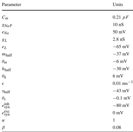
Table 2 Model parameters
Parameter Units
Cm 0.21pF
gNaP 10 nS
eNa 50 mV
gL 2.8 nS
eL −65 mV
mhalf −37 mV
θm −6 mV
hhalf −30 mV
θh 6 mV
0.01 ms−1
shalf −43 mV
θs −0.1 mV
einhsyn −80 mV
eexcsyn 0 mV
α 1
β 0.08
whereVidenotes voltage,hithe inactivation of the persistent sodium currentINaP,si the fraction of the maximal synaptic conductance that is induced by the population’s activity, and s the vector ofsvariables of all populations in the network (although the evolution ofVi does not depend directly onsi). In the voltage equation for popula-tioni,INaP(Vi, hi)=gNaPm∞h(Vi−eNa),IL(Vi)=gL(Vi−eL)is a leak current,
Isyn(Vi, sj)=gsynij sj(Vi −esyn)for esyn∈ {eexcsyn, esyn}inh denotes synaptic current
in-duced by populationj,Iext(Vi)=(iiext)(Vi−eexcsyn)denotes excitatory synaptic current
with conductanceiiextfrom a source outside the network,m∞,h∞, ands∞are mono-tone sigmoidal functions given byx∞(v)=(1+exp((v−xhalf)/θx))−1,x∈ {m, h, s} withm∞ands∞increasing andh∞decreasing, andτh(v)=cosh((v−hhalf)/2θh) for 0< 1. All synaptic inputs are defined with gijsyn>0; whether a synaptic
input is excitatory or inhibitory is determined by its reversal potentialesyn. Default
parameter values used in simulations are listed in Table2; values ofiiext are varied and are discussed as they arise in our analysis. Simulations of the above system give physiologically realistic voltage ranges with the parameters used in Table2. How-ever, because we are interested in relative durations of activity, it is more useful to consider rescaled voltage as a representation of population activity. That is, the popu-lation activity, PA, is related to voltage,V, as follows: PA(V )=1/(1+e(V+30)/−2). This can be seen in Figs.6,15, and16.
With these parameter values, our model equations satisfy several structural hy-potheses. We base our analytical arguments on these hypotheses, so that our results extend beyond our specific choices of model functions and parameter values.
(H1) For each population i, for all relevant synaptic inputs s, the Vi nullcline,
Fig. 3 Nullcline configurations for varying values ofθh(shifting thehnullcline, red) to illustrate key
structures in phase space
V=Vi,L(h,s), V =Vi,M(h,s), and V =Vi,R(h,s) withVi,L< Vi,M< Vi,R
for each(h,s)for which all three exist. For our choice of model, for fixed s,
Vi,LandVi,R increase as a function ofhandVi,M decreases as a function of h, so this will henceforth be assumed as well, although it is not required for our results to hold. Figure3illustrates these structures and those introduced in subsequent hypotheses.
(H2) For each populationi, thehi nullcline,{(Vi, hi):gi(Vi, hi)=0}, is monotone decreasing.
(H3) In the absence of synaptic coupling (gsyn=0), each population has a unique
fixed point,pi,FPR(0)=(Vi,FPR(0), hFPi,R(0)), on the right branch of theVi nullcline for a range of input conductances,iiext.
(H4) In the presence of coupling (gsyn>0) and with input strengthiiextfixed within the range we consider, the right fixed point is retained and left pi,FPL(s)= (Vi,FPL(s), hFPi,L(s)) and middle pFPi,M(s)=(Vi,FPM(s), hFPi,M(s)) fixed points are gained and lost via saddle-node bifurcations that occur for some nonzero choices of the synaptic input s (for example, see Fig.4).
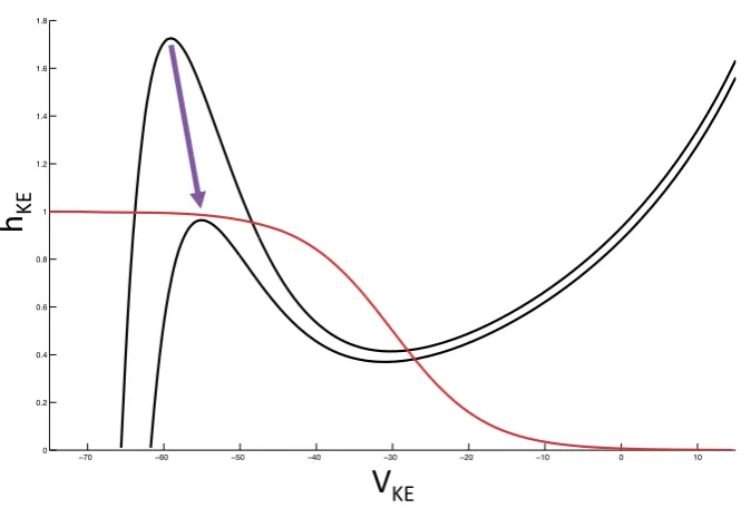
Fig. 4 Saddle-node bifurcation for KE. The red curve is thehKEnullcline, while the black curves are
VKEnullclines for differing combinations of synaptic input. The change between these two combinations
induces a saddle-node bifurcation. We illustrate this bifurcation in the(VKE, hKE)phase plane since it is
critical for delaying KE activation in the rostral rhythm
population is intrinsically tonically active (Fig.3, right fixed point). In our desired network activity, bursting behavior in a population of neurons consists of regular al-ternations between states of low voltage near some family of left nullcline branches
Vi,FPL(s)(silent phase) and states of tonic spiking (i.e., elevated voltage) near some family of right nullcline branchesVi,FPR(s)(active phase), linked via abrupt voltage transitions of significant amplitude, corresponding to jumps between branches. In this framework, the synaptic decay must be sufficiently slow relative to the time scale of voltage jumps, to avoid convergence to a fixed point. Since the synaptic variables represent conductances induced by populations of neurons that are generating a burst of activity, the assumption that they decay gradually during a phase is quite reason-able. On the other hand, we take synaptic activation to occur on the fast time scale, reflecting the synchronized onset of activity in a presynaptic population; see Eqs. (2) and (3) below.
A key point is that hypotheses (H3) and (H4) together imply that transitions from the silent to the active phase must occur by escape. Given a mutually inhibitory pair of populations where one is active and the other is silent, the silent population may become active by reaching the jump up (left) knee of itsV nullcline (i.e., left fold of its family ofV nullclines, parameterized by the synaptic strengthscontrolled by the other population). Doing so allows it to jump to the active phase, inhibiting the other population and, for sufficiently largegsyn, relegating the other population to
popu-lation [25,26]. Thus, in addition to the surfaces of fixed points for each population,
pFPi,X(s)=(Vi,XFP(s), hi,XFP(s)),X∈ {L,M,R}, of mathematical importance are also the surfaces of jump up and jump downV nullcline folds, or knees, for each population:
(ViJU(s), hJUi (s))and(ViJD(s), hJDi (s)). For fixed levels of external and synaptic in-puts, the jump up (down) knee corresponds to a local maximum (minimum) of theVi nullcline. A surface of knees is then the surface of these local extrema, parameterized by the values of the synaptic input variables, for a fixed external input strength.
Based on our parameter choices (Table2), for each i, we consider that jumps between branches of aV nullcline occur instantaneously relative to the rate ofINaP (de)inactivation and relative to the slow decay ofsi (set by the small value ofβ) in the silent phase. Furthermore, we have performed simulations with a very steep synaptic activation functions∞(v), sinceθs is quite small. Thus, for purposes of analysis, we writeβ=β˜, defineτ =t, and let a prime denote differentiation with respect toτ. We then extract from system (1) in the→0 limit a fast subsystem governing jumps between phases:
CmV˙i=Fi(Vi, hi,s), j=i,
˙ hi=0,
˙
si=α(1−si)s∞(Vi),
(2)
a slow subsystem governing evolution within the silent phase:
hi=gi
Vi,L(hi,s), hi
,
si= − ˜βsi,
(3)
and a slow subsystem governing evolution within the active phase
hi=gi
Vi,R(hi,s), hi
,
si=1.
(4)
At any time when there is no population making a fast jump, the collection of popula-tions evolves in a high-dimensional slow phase space with governing equapopula-tions given by making an appropriate choice of either Eq. (3) or Eq. (4) for each population.
Suppose we consider a collection ofN interacting populations. Sincesi does not affectVi,hi directly, it is useful to project the trajectory to anN-dimensional slow phase space for each population, with dimensions corresponding to that population’s
hvariable along with thesvariables for the otherN−1 populations. The population’s jump up and jump down knees,(ViJU(s), hJUi (s))and(ViJD(s), hJDi (s)), are then given by surfaces in its slow phase space (e.g. [27,28]).
3 Results
3.1 Baseline Simulation Results
We simulated system (1) using XPPAUT [29] to find parameter values for which the network (Fig. 2, right) would generate a rostral scratch rhythm under one set of constant external input strengths,{iiext}R, and a pocket scratch rhythm under a different set of constant external input strengths,{iiext}P (see Fig. 1). We required that synaptic weights,{gsyn}ij , were fixed at the same values for both rhythms, such that our results would represent activation of a fixed network by two different forms of stimulation, presumably representing effects of body surface stimulation in two different regions (Fig.1).
Two distinct classes of synaptic weights were implemented in the network, stan-dard (S) and strong cross-excitation (SCE) (Fig.5). The S class is based on the idea that a rostral-inducing stimulus should strongly recruit the excitatory ER pool respon-sible for driving HF and less strongly recruit the inhibitory IR pool that blocks this action, and similarly for pocket. These input levels can also be interpreted as all four interneuron populations receiving a baseline level of input, with ER, IP receiving additional input in rostral and EP, IR receiving additional input in pocket.
The SCE class is based on the reasoning that the entire rostral pool, including both ER and IR, should be most strongly stimulated by rostral-inducing stimuli, and sim-ilarly for pocket. We call this weight class SCE because a stronger cross-excitation from ER to IP and from EP to IR (0.8 nS versus 0.5 nS) was used to promote syn-chrony between these pairs of populations in this case. Here, all four interneuron populations can be viewed as receiving a baseline level of input, but with an addi-tional input boost to the “active side”.
In both cases, the synaptic weights at the interneuron level (not to the MNs) are just a minimal combination that allows oscillations to occur; that is, decreasing any of the weights appreciably without changing the others to compensate leads to a loss of all oscillations. The baseline input strengths (0.17 nS in S and 0.16 nS in SCE) were chosen such that no oscillations are elicited when no interneuron populations receive an additional drive. The S and SCE weights are similar in the sense that they result in qualitatively similar interneuron dynamics and output from the interneurons to the MNs. This output is largely constrained by the required behavior of HF and HE:
• HF and HE activate in antiphase and do not receive temporally overlapping exci-tation and inhibition [2–4] meaning that IP must be in antiphase with EP and IR in antiphase with ER (Fig.2, right panel).
• In light of these antiphase relations, it is natural for EP, IR to activate in synchrony and ER, IP to activate in synchrony.
• HF is activated longer than HE in rostral (Fig.1, right panel of Fig.2, Fig.5), hence ER must receive more input than EP in rostral (reversed in pocket).
Fig. 5 Synaptic weights and
input strengths. Two different sets of synaptic weightsgijsyn
and external input strengthsiexti
used in our simulations of system (1), with units (mS) omitted. Top: “standard” weights; bottom: “strong cross-excitation” weights. Solid
lines ending in circles denote
inhibitory connections; dashed
lines ending in arrows represent
excitatory ones. Both sets of weights include certain symmetries but the activity they support is robust to asymmetric perturbations
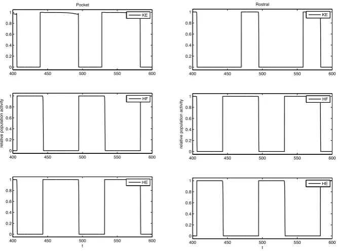
Fig. 6 Basic simulation results. Example relative population activity for MN populations resulting from
simulation of system (1) with the S weights. MN population identified in the legend. The y-axis represents population activity as rescaled voltage, 0 indicates silent, 1 indicates active. Note that the relative timing and durations of activity in the simulation match the recordings (see Fig.1). The SCE weights produce the desired relative timing and durations as well (not shown)
3.2 Necessary Conditions for Rhythms
Because hip extensor and hip flexor each only receive antiphase excitation and in-hibition and maintain the same antiphase relationship with each other across both rhythms, choosing synaptic weights from the interneuron populations to HE and HF is easy. We henceforth assume that these weights and the weights within the interneuron network are fixed such that this antiphase behavior, with appropriate rel-ative phase durations, occurs. Because KE receives temporally overlapping excitation and inhibition, synchronizes with a different hip component in each rhythm, and ex-hibits a delay in onset relative to its hip partner in rostral and not pocket, the synaptic weights to KE are much more constrained. We will consider dynamics in certain slow phase spaces to derive conditions on these weights that yield multi-functionality of the networks shown in Fig.5, which generalize to any model with a qualitatively similar structure.
3.2.1 Reduction of Slow Phase Space Dimension
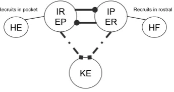
Fig. 7 Reduced module controlling knee extensor activity. Two interneuron units form a half-center
oscil-lator, linked by mutual inhibition (thick solid lines). Each unit recruits a corresponding hip MN (thin solid
lines) and supplies a hybrid excitatory and inhibitory input to KE (dot dashed lines with squares), with a
single corresponding synaptic conductance variable
activate on the fast time scale (Eq. (2)) and decay on the slow time scale (Eq. (3)). Additionally, the inactivation of persistent sodium for KE,hKE, evolves on the same
slow time scale. Therefore, there is a five-dimensional slow phase space for KE. An-alyzing dynamics in this full, five-dimensional space is impractical.
To reduce dimension further, we identify the interneuron pairs that activate to-gether,(EP,IR)and(ER,IP), to form a single half-center oscillator and we consider a reduced model to describe KE activity, illustrated in Fig.7. With this reduction, us-ingesynexc=0,sER=sIP, andsEP=sIR, the synaptic input for knee extensor becomes
IsynKE=sER
(gIP+gER)VKE−gIPeinhsyn
+sEP
(gIR+gEP)VKE−gIResyninh
.
This step reduces our phase space from five dimensions to three, with variables
(hKE, sEP, sER). The projection of the periodic pocket trajectory of the reduced model
to(hKE, sEP, sER)space is shown in the top left of Fig.8, along with several curves
that are important for understanding KE dynamics. These plots are critical to our analysis. When ER is active,sER≈smax, so the corresponding part of the trajectory,
color coded red, lies approximately on the{sER=smax}plane within phase space,
which is the back right face of the cube shown. Similarly, the epoch with EP active hassEP≈smaxand yields a trajectory, color coded black, near the back left face of
the cube. As an alternative to considering a three-dimensional phase space, however, it is convenient to switch between a pair of two-dimensional slow phase planes, cor-responding to the back two faces in the top left of Fig.8, as EP and ER alternate between periods of silence and activity. These are shown in the top right of Fig.8. For example, while EP is active,sER evolves and the projection of the trajectory to
the (hKE, sER)plane is shown as the thick black curve. Of course, even after EP
switches from active to silent, the projection of the trajectory to the(hKE, sER)plane
still exists; the projected trajectory segment after the switch is shown as the thin black curve. Using similar considerations for the projection to(hKE, sEP), we in fact plot
two copies of the full trajectory, each in its own two-dimensional phase plane, one with the trajectory shown thick while EP is active and thin while ER is active, and the other the opposite. The switch from EP active to ER active occurs abruptly when
sEPbegins its slow decay fromsmaxandsERincreases very rapidly (instantly in the
singular limit) tosmax, and we switch each curve from thick to thin whensEP=sER
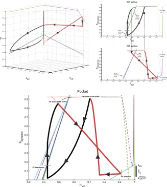
Fig. 8 Phase space views for the KE dynamics in the reduced module shown in Fig.7during the pocket rhythm. Top left: full three-dimensional slow phase space. Top right: projections onto the two two-dimen-sional planes where the trajectory lies. Bottom: single, combined two-dimentwo-dimen-sional representation. In all plots, black and red curves are projections of parts or all of the trajectory of a periodic pocket scratch solution, with bold black and thin red denoting times when EP is active and bold red and thin black times when ER is active. Green curves denote the fixed point curves for KEpFPKE,R(s)(stable, solid),pFPKE,M(s)
(unstable, dashed), andpFPKE,L(s)(stable, solid) (in order of increasinghKE) while EP is active. Magenta
curves denote the analogous curves of fixed points for KE while ER is active. The dark blue curve is the
curve of jump down knees for KE while EP is active; cyan curves are jump down knees and jump up knees (largerhKEvalues) for KE while ER is active. Finally, dashed black curves in the top right indicate points
Finally, since the values over whichsERandsEPvary over each period are similar,
both slow phase planes can be compressed to a single plot. Again, when this plot is displayed in the bottom part of Fig.8, we show two copies of the trajectory. For the black (red) copy,sdynamicshould be interpreted assER(sEP), with thick and thin parts
as in the separate two-dimensional plots (thick black when EP is active such thatsER
decays gradually, thick red when ER is active such thatsEPdecays gradually).
For fixed input levels(sEP, sER), theVKEnullcline has one or more fixed points, a
jump up knee, and a jump down knee. These become two-dimensional surfaces under variation of both inputs, while fixing one input at smax selects a one-dimensional
curve. In Fig.8, the curves of fixed points forsEP=smaxare shown in green and for sER=smaxin magenta; both show up in the bottom plot, but it is important to keep
in mind that each is only meaningful whensdynamic has the correct interpretation.
Similarly, the curves of knees are shown in dark blue and cyan. There are two cyan curves, with smallerhKEvalues for jump down knees than for jump up. There is only
one dark blue curve because the curve of jump up knees is outside of the relevant range of(hKE, s)values when EP is active.
3.2.2 Scratch Trajectories and Weights of Synapses onto KE
To generate pocket and rostral scratch rhythms in our model, we had to select val-ues for synaptic connections in the model network, which remain the same for both rhythms, and strengths of external inputs to the network, which differ between the rhythms. As mentioned previously, fixing the weights of synapses to the HE and HF MNs is not particularly interesting, since the desired antiphase activation patterns for each rhythm are set at the interneuron level in the full or reduced model. For conve-nience, we simply choosegsynHE,EP=gsynHF,ERandgHEsyn,IP=gsynHF,IR.
The weights of synapses onto KE are more interesting. To understand how these are constrained, we can focus on the reduced model, which maintains four distinct synaptic weights from the interneurons onto KE. With the convenient viewpoint that we have established, it is now helpful to consider the details of the trajectories for pocket scratch (Fig.8) and rostral scratch (shown in Fig.9in a two-dimensional view analogous to the bottom panel of Fig.8) for our baseline parameter choices. Recall that in the pocket rhythm, KE activates with HE, here represented by the activation of EP. When EP becomes active and the thick black part of the trajectory starts,hKE
decreases, corresponding to the trajectory being in the active phase for KE, near a right branch of theVKEnullcline. The trajectory cannot cross the curve of jump down
knees (dark blue) withsdynamic decreasing, because it is blocked by the green fixed
point curve (which almost coincides with the dark blue one in Figs.8 and9). The switch ofsdynamicfrom decreasing to increasing corresponds to the activation of ER
(and hence HF). The rise in sdynamic pulls the trajectory across the curve of jump
down knees of the VKE nullcline (dark blue), terminating the active phase of KE.
We then switch our view to the thick red trajectory, along whichhKEincreases (and
sdynamic=sEPdecreases), corresponding to the trajectory being in the silent phase for
KE, near a left branch of theVKEnullcline. The trajectory actually reaches the curve
Fig. 9 Rostral slow phase plane. Trajectory for KE for rostral scratch projected to a single slow phase
plane. Coloring of curves is identical to Fig.8. Bottom: zoomed view near the saddle-node bifurcation where the fold in the magenta fixed point curve intersects the cyan jump up knee curve for ER/HF active
yielding a rise insdynamic, and we switch back to the thick black trajectory, where
we started. In fact, experiments reveal a natural variability in pocket scratch patterns. There are many experimental examples of pocket rhythms in which knee extensor becomes active just before hip extensor, at the final moments of hip flexor activity, and indeed a mean pocket rhythm computed from experimentation has this property [30]. Hence, this result provides validation that the solution that we have obtained provides a reasonable reduced representation of a pocket rhythm.
In the rostral rhythm, KE activation follows that of HF, here represented by the activation of ER, with a delay. When ER becomes active, and the thick red part of the trajectory starts, KE is still in the silent phase, with a fixed point on the left branch of theVKEnullcline (solid magenta line at the far right of Fig.9; see especially the
bottom panel of Fig.9). Assdynamic decreases, the trajectory approaches the
a saddle-node bifurcation (meeting the dashed fixed point branch in the figure) at the curve of jump up knees of theVKEnullcline (lower right cyan curve; also see Fig.4).
At the bifurcation, KE activates andhKEstarts to decay, with the trajectory heading
toward the magenta curve of fixed points in the left part of Fig.9. When the activity of ER terminates,sdynamicincreases, which pulls the trajectory through the curve of
jump down knees (cyan) and hence switches KE to the silent phase. With EP now activated (thick black part of the trajectory) and KE silent,hKEincreases, but there is
no curve of jump up knees available to reach over the relevant range of(hKE, sdynamic)
(note the absence of a dark blue curve in the lower right of Fig.9, analogous to its absence in Fig.8). Thus KE remains silent until the active phase of EP ends,sdynamic
rises, and ER activates at the transition from the thick black to the thick red part of the trajectory, where we started.
From our investigations, it appears that obtaining both pocket and rostral scratch rhythms with the same set of synaptic weights through the dynamic mechanisms we have described requires certain phase plane features and timing relations, which arise in the trajectory descriptions we have provided. Classifying these in terms of particular phases of rhythms, the requirements on the trajectory projected to KE space are as follows:
(i) pocket, EP active: the trajectory must not reach the curve of jump down knees assdynamic decreases yet must cross it assdynamic rises (Fig.8, the red part of
the trajectory does not increase through the cyan curve but the black part of the trajectory increases through the blue curve);
(ii) pocket, ER active: the trajectory must reach the curve of jump up knees as
sdynamic decreases, but only sufficiently late in the active phase of ER (Fig. 8,
the red part of the trajectory reaches the right cyan curve near where it switches to black);
(iii) rostral, ER active: the trajectory must follow a curve of fixed points to a saddle-node bifurcation at the curve of jump up knees, must subsequently not reach the curve of jump down knees assdynamicdecreases, and must cross the jump down
knees assdynamicrises (Fig.9, red parts of the trajectory);
(iv) rostral, EP active: the trajectory must not reach the curve of jump up knees as
sdynamic decreases (Fig.9, note that there is no curve of jump up knees visible
while EP is active, corresponding to the black part of the trajectory).
The first part of requirement (iii) is critical for imposing a delay between ER ac-tivation and KE acac-tivation. Requirement (iv) goes together with (iii); certainly no delay would be possible if the trajectory reached a curve for the activation of KE even before ER activated at all! To achieve requirements (iii) and (iv), we find that it is necessary but not sufficient forgKEsyn,EP,gsynKE,IP,gKEsyn,ER,gsynKE,IRto be such that
both requirements (i) and (iii) are partially trivial, since the trajectory is blocked from reaching jump down knees by the location of fixed point curves. Nonetheless, they do constrain weights to ensure thathKEdecays sufficiently during each active phase
such that subsequent rises insdynamiccan pull the trajectory across the curves of jump
down knees, transitioning KE to the silent phase along with its interneuron partner, as desired.
3.2.3 Conditions for Rhythm Selection and Slow Phase Plane Analysis/Contraction Arguments
With our synaptic weights onto KE and slow phase plane structure fixed to satisfy the requirements described in the previous subsections, for each rhythm, we now de-rive certain conditions on the set of inputsI= {iIPext, iEPext, iERext, iIRext}, which ensure that that rhythm will be selected. Some of these conditions are necessary, while together the collection is sufficient, although we cannot rule out that there may be different necessary and sufficient conditions elsewhere in parameter space. At a minimum, it is always necessary that the inputs actually elicit oscillations, both at the interneuron and the motoneuron levels. For convenience in what follows, defineTactivej (I )as the length of time for which populationj is active for a given set of input parametersI
as above.
Recall that we have defined a slow phase plane structure in which activation oc-curs by gaining access to the curve of jump up knees with ER active (as discussed in the previous subsection). For simplicity, we henceforth refer to sdynamic as s. We
define the interval Is = [sERmin(I ), sSN]. sSN is defined as the value of s at which
the saddle-node bifurcation of fast subsystem critical points occurs with ER active (Figs.8and9), andsERmin(I )is simply the minimum value to whichsdecays while EP is still active. The dependence ofsminER on input arises because the setI determines how long EP and ER are active and hence how fars decays fromsmax. The interval Is is illustrated for a particular input setI in Fig.8.
When there is a switch between EP active and ER active,s jumps tosmax. (This
occurs instantaneously in the singular limit, but in our simulations, such as Figs.8 and9, the switch occurs at some s∗ < smax. The value of s∗ can easily be
ap-proximated as s∗≈smaxe−βt where, using the differential equation for s in (1), t satisfies smaxe−βt =(smin(I )−smax)e−(α+β)t+smaxgiven the minimal value of sdynamic is smin(I ). This equality illustrates how t →0 and hence s∗→smax as α→ ∞, corresponding to a complete separation of time scales.) We assume that
hJDEP(smax)=hERJD(smax)and denote thish-value byhmax. This assumption is based on
the numerical observation that the curves of right knees corresponding to EP active or ER active are quite close, which relates to the reversal of synaptic excitation at large voltages, and appear to converge ats nearsmax. We define a second interval Ih= [hmin(I ), hmax], wherehmin(I )is the value ofhKEalong the ER curve of jump
down knees at s=sERmin(I ). This interval specifies the full set ofhKE values from
which a jump down will yield a crossing of the curve of knees. The intervalIh is illustrated for a particular input setI in Fig.9.
Fig. 10 Pocket rhythm:
duration and timing of MN activations in simulations (left) and experimental recordings from MNs (right). Recall that
HF activates with ER and HE
with EP
toTactiveER (I ) < TactiveEP (I ). In a successful pocket rhythm, KE activation can occur at any value ofsdynamic=sER∈Is. The closer tosERmin(I )that activation occurs, the less
the overlap of KE and HF activations. With the above constraints and definitions, the pocket rhythm will exist for any set of inputs for whichIs is mapped to int(Is)under the slow flow pieced together by appropriate selection of (3) and (4). This mapping to the int(Is)helps ensure that requirement (ii) in the previous section is met, as we will show below.
By continuity, it is sufficient for the existence of a stable pocket rhythm to find conditions onI under which the endpoints sSN and sminER(I ) are mapped into
the interior of Is. We use slow phase plane arguments to do so. Fix input set I. Note that there is an ordering of the trajectories starting from the relevant part of the cyan curve of jump up knees corresponding to ER active (Fig. 8), given by LKIs := {(hKE, s):s∈Is, hKE=h
JU
ER(s)}. That is, suppose(h1, s1), (h2, s2)∈LKIs withh1> h2and hences1> s2. Flow(h1, s1)forward under (3), obtaining a
trajec-tory(h1(t ), s1(t )), untils1(t )=s2. Similarly, denote the forward flow from(h2, s2)as (h2(t ), s2(t )). Ifh1(t ) > h2(h1(t ) < h2), thenh1(t+τ ) > h2(τ )(h1(t+τ ) < h2(τ ))
for allτ untils1(t+τ )=s2(τ )=sERmin(I )and the ER active phase ends. Moreover,
by continuity, all points on LKIs are ordered in this sense.
Thus, the trajectory from LKIs that attains the minimal h(s) value when s=
sminER(I )when evolved forward in time is either the one starting froms=sSN
(cor-responding to<in the statements above) or that from s=sminER(I )(corresponding to>). It turns out that the more interesting case, for which our argument yields one additional sufficient condition, occurs when the minimalhcorresponds to the initial conditions=sSN, with the initial value ofhgiven byhSN:=hJUER(sSN), so without
loss of generality we henceforth assume that this orientation holds (Fig.11). Now, letT (I )=(1/β)ln(sSN/sERmin(I ))denote the time fors to decay fromsSN
tosERmin(I ). Suppose we choose an initial condition such that KE activation occurs at
s=sSN during the ER active phase. We introduce the notationh(a;b, c) to denote
thehKE value at timea for a trajectory that started at time 0 with initial condition
(hKE, s)=(b, c). The first sufficient condition that we include is that the resulting
KE trajectory does not cross a curve of jump down knees when EP takes over from ER:
(P1) h+SN:=hT (I );hSN, sSN
> hmax.
Fig. 11 Useful trajectories for deriving sufficient conditions for a stable pocket rhythm. Solid black lines
are flows forward from a known point. Dotted black lines represent backward flows. Left: the conditions that arise when a flow is initiated fromsSN. Right: the conditions that arise when a flow is initiated from sERmin(I )
start of the EP active phase, wherehminER(I ):=hJUER(sERmin(I )), and evolves under (3) with EP active for timeTactiveEP (I )(to{s=sEPmin(I )}). The condition (Fig.11, right) is
(P2) hTactiveEP (I );hminER(I ), smax
< hmax.
Next, we obtain two conditions that are sufficient to ensure that the flow of LKIs yields trajectories that return to int(LKIs)and that do so while ER is active, but not newly active (to ensure requirement (ii) in the previous section). To state these con-ditions, we need to make use of the backwards flow of the endpoints(hSN, sSN)and (hJUER(sERmin(I )), sERmin(I ))back to the line {s=smax} under system (3) with ER ac-tive. Denote theh-coordinates of these intersections byh−SNandh−s
min, respectively,
withh−s
min< h
−
SNby continuity. Recall that the forward trajectory from the endpoint (hSN, sSN)has h=hSN+ :=h(T (I );hSN, sSN)when EP becomes active (see
Con-dition (P1) and Fig.11, left). With these definitions, the final sufficient conditions, which guarantee that the next KE activation occurs from int(LKIs), read
(P3) hTactiveEP (I );hminER(I ), smax
< h−SN,
(P4) hTactiveEP (I );h+SN, smax
> h−s
min.
(P1)–(P4) are conditions on relative orderings of points in the slow phase space that may result under certain choices ofI. To appreciate that whenI is chosen to satisfy Conditions (P1)–(P4), together with the earlier condition that TactiveER (I ) < TactiveEP (I ), it follows that LKIs is mapped into its own interior under the flow and there exists a stable periodic pocket rhythm, note that the time of evolution from
s=smax down to s=sERmin(I ) under (3) with EP active is exactly timeTactiveEP (I ).
Conditions (P3)–(P4) ensure that all trajectories emanating from LKIs end up with
h∈(h−min, h−SN)when ER first activates. From the time of ER activation, these trajec-tories all evolve under (3) froms=smax, and Conditions (P3)–(P4) imply that they
reach int(LKIs). In particular, they arrive withs > s
min
times that are less thanTactiveER (I ), before the end of the ER active phase, as desired. Furthermore, Condition (P3) allows us to clarify what we mean by “sufficiently late” in requirement (ii) from the previous section. That is, the time KE spends in the silent phase is minimized when it activates from(hSN, sSN), or equivalently when it enters
the silent phase ath=h−SN. We can use Eq. (3) to calculate the minimal time spent in the silent phase:t∗=−β1ln(sSN
smax). (P3) guarantees that ER is active for at least time
t∗before KE activates.
In summary, we conclude that for a choice of synaptic weights such that our earlier assumptions on the structure of phase space are satisfied, for any choice ofIsuch that Conditions (P1)–(P4) hold, there exists an open set of initial conditions supporting a stable, periodic pocket rhythm. Choices of weights that shrinksSNtowardsERmin(I ),
narrowingIs, yield less overlap between the phases when KE and HF are active at the end of the ER active phase, and hence more experimentally realistic solutions. This change can be achieved, for example, by weakening the excitation from ER to KE relative to the inhibition from IP to KE; however, making this excitation too weak will prevent KE activation entirely and destroy the rhythm.
Rostral Rhythm Next, recall the form of the rostral rhythm, illustrated in Fig.9. Since HF is active longer than HE in this rhythm, we takeiEPext< iERext, which leads to
TactiveEP (I ) < TactiveER (I ). In the rostral rhythms that we seek, we assume that KE acti-vation occurs withsdynamic=sSNwith ER (and thus HF) active, in order to achieve
the delay with respect to HF activation in a robust way, keeping the same synaptic weights as in the pocket case. We also require that KE activation ends at the same time as ER activation. We now use slow phase plane arguments to derive sufficient conditions for the existence of a stable rostral rhythm that meets these constraints.
The trajectory for the desired rhythm should reach the curve of jump up knees withs=sSNand ER active and flow from there to the intervalIh. Using our previous
definitions of T (I ) and hSN, a sufficient condition to achieve this requirement is
simply (Fig.12):
(R1) hT (I );hSN, sSN
∈Ih.
Next, it suffices to impose conditions under which the flow maps the intervalIh back to the curve of jump up knees where it intersects{s=sSN}at some time after ER has already activated but while ER is still active. To derive these, it suffices to consider the trajectories generated by the forward flow from the endpoints of Ih, namely(hmin(I ), sERmin(I ))and(hmax, sERmin(I )). There are two aspects to this mapping
requirement. One is that all trajectories have time to reach{s=sSN}from{s=smax}
(Fig.12), a condition for which can be written in two equivalent forms using the notation we have introduced:
(R2) sSN> sERmin(I ) ⇔ T ER
active(I ) > (1/β)ln(smax/sSN).
The other aspect is that even the trajectory with minimalhvalue, which originates from(hmin(I ), sERmin(I ))just before EP activates, must be able to reach (hSN, sSN)
Fig. 12 Useful trajectories for
deriving sufficient conditions for a stable rostral rhythm. The solid
black line denotes the flow
forward from(hSN, sSN).
Dashed black lines indicate
flows forward from two points
(hmax, sSN)and(hmin(I ), sSN).
The dotted black line represents
a backward flow
EP active, say to(hEP, sEP), and then continues forward under (3) with ER active
from(hEP, smax)(Fig.12). Our additional sufficient condition is therefore
(R3) hEP> h−SN,
whereh−SNis derived from the backwards flow of (3) with ER active as in the previous subsection.
Conditions (R1)–(R3), together with the earlier condition that TactiveEP (I ) < TactiveER (I ), are sufficient for all initial conditions withinIhto pass through(hSN, sSN),
in the singular limit, albeit at different times, and reach the interior ofIhwith ER ac-tive, which guarantees a stable rostral rhythm. We observe that our strong structural requirement that KE activation occurs at a saddle-node bifurcation of fast subsystem equilibria, which ensures a robust delay of KE activation relative to ER (and hence HF) activation as seen in the rostral rhythm, makes our remaining sufficient condi-tions for the existence of a stable rostral rhythm milder than those we invoked to ensure the existence of a stable pocket rhythm.
Key Differentiator Between Rhythms The work in this section supplies a variety of conditions on the relative positions of various trajectories such that when a set of inputs allows an appropriate collection of conditions to be satisfied, a pocket or rostral rhythm results. From this analysis and our numerical simulations, we can extract a key factor that distinguishes whether a rhythm generated by an input set is likely to be a pocket rhythm or a rostral rhythm. Given an initial condition on LKIs with ER active,
• inputs that lead tohKE> hmaxat the termination of ER activity push the solution
toward pocket;
• inputs that lead tohKE< hmaxat the termination of ER activity push the solution
Fig. 13 Key differentiator. The location of a trajectory at the end of the ER active phase, relative tohmax,
ends up being the key separator in the slow phase plane between inputs that elicit rostral and those that elicit pocket
In other words, roughly speaking, the rhythm is selected based on whether or not the KE trajectory has access to a curve of jump down knees from which to enter the silent phase at the switch from ER activity to EP activity (Fig.13). Of course, this access depends on the time remaining with ER active after KE activates, which in turn depends on all relationships presented in the previous two subsections. Nonetheless, a numerical exploration of this timing issue can give a quick, rough idea of which solutions will be favored for a given input set, an option that would not have been obvious without our analysis. Further, this analysis provides a framework in which features can be examined thoroughly, which we harness in the next section.
3.3 Modeling Additional Experimental Results
3.3.1 Experiments and Simulations with Input Switching
We can test the experimental relevance of our model by trying to simulate some additional experiments that have been performed involving the rostral and pocket rhythms. Furthermore, now that we understand the dynamic mechanisms underlying each rhythm and the rhythm selection process, we can understand the outcomes of simulations in these scenarios.
Fig. 14 Currie and Stein 1988 experiments. Converting a rostral rhythm to a pocket rhythm. Bottom three
traces show MN activity corresponding to KE, HF, and HE, respectively. Initial bouts of activity represent
a rostral rhythm with large delay of KE activation relative to HF. Transient pulse stimulation of the VPP nerve (inverted triangles) eventually switches the network into a pocket rhythm. Figure source: [31]
Fig. 15 Simulation of Currie and Stein 1988 experiments. A switch from rostral inputs to pocket inputs,
at the time indicated by the arrow, causes the model behavior to transition from rostral to blended out-put to pocket. Standard weights were used, with similar results obtained for SCE weights (not shown). Inputs:Irostral= {iIP=0.19, iEP=0.17, iER=0.19, iIR=0.17}, Ipocket= {iIP=0.17, iEP=0.19,
iER=0.17, iIR=0.19}
To qualitatively reproduce this experiment, we consider the result of an instanta-neous switch of inputs. That is, a rostral input set,Irostral, is given to the system. After
several periods, at the end of a phase of HE activity (as in the experiment), the in-puts are switched to a pocket input set,Ipocket. With both the Standard and the Strong
Cross-Excitation synaptic weights, this change in inputs leads to a similar transition to pocket as seen in the experiment (Fig.15). Our phase plane analysis makes it easy to understand the switch in dynamics. Once pocket inputs are applied, KE still reaches the SN bifurcation and activates while EP and HF are active, as in rostral. But the pocket inputs shortenTactiveER (I ), allowing EP and hence HE to take over before
hKEdecays down tohmax. Thus KE remains active when EP/HE activates, yielding
a cycle that blends features of rostral and pocket followed by rapid convergence to a pocket rhythm.
Fig. 16 Pocket to rostral simulations. Applying rostral inputs during a pocket rhythm may or
may not induce a switch to rostral. A pocket rhythm was induced using Ipocket= {iIP=0.17,
iEP=0.19, iER=0.17, iIR=0.19}. Inputs were switched at the time indicated by the arrows to one
of two different input sets, each of which evoked rostral from rest. Top:Irostral1 = {iIP=0.19, iEP=0.18,
iER=0.19, iIR=0.18}maintains the pocket rhythm, and hence uncovers bistability in the system.
Bot-tom:Irostral2 = {iIP=0.19, iEP=0.17, iER=0.19, iIR=0.17}leads to switching behavior as seen in
experiments [31]
HE, unlike the prototypical pocket rhythm (Fig.16, top). In the other case, the rostral inputs cause a switch to the rostral rhythm (Fig.16, bottom).
In the case where pocket persists, we conclude that the rostral inputs that are ap-plied render the system bistable. These inputs are closer toIpocketthan are other
ros-tral inputs that do not reveal bistability. In particular, the stronger inputs to IR and EP in the former case cause an earlier switch from HF to HE, allowing pocket dynamics to be maintained. In the SCE set up, we do not observe bistability numerically across a wide range of inputs and synaptic weights that we have explored.
3.3.2 Explanation of Bistability (and Lack Thereof)
The selection between the two cases illustrated in Fig.16essentially comes down to a race between EP (corresponding to HE) and KE: from the activation of ER/HF, does EP reach the jump up knee beforehKEis able to decay to reachhmax? If EP does
ac-tivate first, then the rhythm remains in pocket. If KE reacheshmaxfirst, then a switch
to rostral can occur. The data used to generate Fig.16indicates that a decrease iniEP
In the SCE regime, we have not observed bistability: introduction of rostral inputs during ongoing pocket switches the rhythm to rostral. Heuristically, we can see why SCE would tend to suppress bistability, based on the SCE synaptic weights (Fig.5). For a pocket rhythm to persist despite rostral inputs, the ER active phase must remain sufficiently short that EP can activate beforehKE drops tohmax(Fig.13). Because
transitions in our networks occur by escape, this requirement means that EP or IR must be able to activate before the ER stays active too long. In SCE, however, the weights of synaptic inhibition from ER to IR and excitation from ER to IP are strong, relative to the S case. These synaptic connections are exactly the ones that would suppress the activation of EP and IR and thus prolong the ER active phase, causing KE to jump down with ER and inducing a switch from pocket to rostral.
3.3.3 Predictions
The observation that some weight and input parameter sets yield bistability and others do not may be useful for making predictions. That is, if bistability is observed exper-imentally, then we can conservatively state that it should rule out certain parameter combinations within the underlying rhythm generating circuit, if indeed that circuit is qualitatively represented by our model. For example, although our simulations were not exhaustive, together with the heuristic arguments we have provided they suggest that an observation of bistability of pocket and rostral rhythms in response rostral in-puts would represent evidence against SCE weights, in which both the excitatory and the inhibitory interneurons projecting to HF are more strongly recruited by rostral stimulation than are the corresponding HE-projecting interneurons.
More generally, we can also observe that if a single circuit generates both pocket and rostral rhythms, then one rhythm may be more resistant to input-induced switch-ing than the other, as we have seen by introducswitch-ing rostral input durswitch-ing an ongoswitch-ing pocket rhythm. This is an important observation: Suppose that two separate modules generated pocket and rostral rhythms. In that case, introducing a rostral input dur-ing ongodur-ing pocket would necessarily recruit the rostral module, likely perturbdur-ing the pocket rhythm in some way that is more significant than seen in our simulations. Hence, bistability may be used to help distinguish between these possible rhythm generation frameworks (see also [5]).
Fig. 17 Effect of input scaling
on phase durations in SCE regime. The black bars represent the durations of the active phases of HE, KE, and HF when the indicated inputs are uniformly decreased by multiplication by a scaling factor less than one, just large enough to maintain each rhythm. The gray bars represent the durations of the active phases of HE, KE, and HF when the scaling factor is greater than one, near the upper bound for maintaining each rhythm
Fig. 18 Effect of input scaling
on phase durations in S regime.
The black bars represent the
durations of the active phases of
HE, KE, and HF when the
indicated inputs are uniformly decreased by multiplication by a scaling factor less than one, just large enough to maintain each rhythm. The gray bars represent the durations of the active phases of HE, KE, and HF when the scaling factor is greater than one, near the upper bound for maintaining each rhythm
INs (Fig.17, right). These results indicate that the escape of the excitatory INs from the silent phase largely controls rhythm frequencies. In fact, we find that the external input to the inhibitory interneurons can be removed and the synchrony patterns of the rhythms (but not the delay in rostral) can be maintained (data not shown), because the excitatory INs still recruit the inhibitory populations to become active. These predictions are more difficult to test, given that these populations of interneurons have not yet been identified, but remain for future experimental consideration.
These differences, in addition to the bistability observed, may serve to differentiate the S regime from the SCE regime in practice.
4 Discussion
It has been postulated that turtle scratching and swimming arise when “behavioral modules” interact and combine to control “muscle synergies” producing appropri-ately coordinated motor outputs [32], but there is a large gap between such an abstract statement and concrete hypotheses about the neuronal networks involved. While a specific wiring diagram for a single circuit that could parsimoniously drive both pocket and rostral scratching has been proposed [4], it is well known that connec-tivity diagrams alone do not uniquely map to output patterns [17]. We have per-formed a computational and mathematical study to investigate whether the proposed unified CPG network, which features only hip-related populations of interneurons, could indeed be responsible for the generation of two different turtle scratch rhythms with distinct knee-hip synchrony patterns. Importantly, these patterns are selected by changing external inputs to the interneurons, with the same synaptic weights between interneurons, and from interneurons to motoneurons, preserved for both. Through the use of slow phase plane arguments, we were able to explain how particular phase space and bifurcation structures underlie the generation of the rhythms and to de-rive sufficient conditions on these structures that guarantee the existence of stable rhythms. This analysis was possible due to time scale decomposition and certain model reductions, despite the relative high-dimensionality of the model system; be-cause our conditions are stated in terms of dynamic structures, they apply beyond the particular model features, such as a slowly inactivating persistent sodium current, used in our simulations. Even with model reductions, the synaptic variables evolv-ing durevolv-ing each stage of each rhythm were hybrid variables, representevolv-ing combined effects of excitatory and inhibitory inputs, which was one unusual aspect of our anal-ysis.