DOI 10.1186/s13408-017-0043-7
R E S E A R C H Open Access
Stable Control of Firing Rate Mean and Variance by
Dual Homeostatic Mechanisms
Jonathan Cannon1 ·Paul Miller1
Received: 27 May 2016 / Accepted: 29 December 2016 /
© The Author(s) 2017. This article is distributed under the terms of the Creative Commons Attribution 4.0 International License (http://creativecommons.org/licenses/by/4.0/), which permits unrestricted use, distribution, and reproduction in any medium, provided you give appropriate credit to the original author(s) and the source, provide a link to the Creative Commons license, and indicate if changes were made.
Abstract Homeostatic processes that provide negative feedback to regulate neuronal firing rates are essential for normal brain function. Indeed, multiple parameters of in-dividual neurons, including the scale of afferent synapse strengths and the densities of specific ion channels, have been observed to change on homeostatic time scales to oppose the effects of chronic changes in synaptic input. This raises the question of whether these processes are controlled by a single slow feedback variable or mul-tiple slow variables. A single homeostatic process providing negative feedback to a neuron’s firing rate naturally maintains a stable homeostatic equilibrium with a char-acteristic mean firing rate; but the conditions under which multiple slow feedbacks produce a stable homeostatic equilibrium have not yet been explored. Here we study a highly general model of homeostatic firing rate control in which two slow variables provide negative feedback to drive a firing rate toward two different target rates. Us-ing dynamical systems techniques, we show that such a control system can be used to stably maintain a neuron’s characteristic firing rate mean and variance in the face of perturbations, and we derive conditions under which this happens. We also derive expressions that clarify the relationship between the homeostatic firing rate targets and the resulting stable firing rate mean and variance. We provide specific examples of neuronal systems that can be effectively regulated by dual homeostasis. One of these examples is a recurrent excitatory network, which a dual feedback system can robustly tune to serve as an integrator.
Keywords Homeostasis·Dynamical systems·Stability·Integrator·Synaptic scaling·Averaging
B
J. Cannoncannon@brandeis.edu
P. Miller
pmiller@brandeis.edu
1 Brandeis University Department of Biology, Volen National Center for Complex Systems, 415
Mathematics Subject Classification (2000) 62P10·92C20·37C10·37C25· 60H10·34F05·37E99
1 Introduction
Homeostasis, the collection of slow feedback processes by which a living organism counteracts the effects of external perturbations to maintain a viable state, is a topic of great interest to biologists [1,2]. The brain in particular requires a precise balance of numerous state variables to remain properly operational, so it is no surprise that multiple homeostatic processes have been identified in neural tissues [3]. Some of these processes appear to act at the level of individual neurons to maintain a desirable rate of spiking. When chronic changes in input statistics dramatically lower a neu-ron’s firing rate, multiple slow changes take place that each act to increase the firing rate again, including the collective scaling of afferent synapses [4, 5] and the ad-justment of intrinsic neuronal excitability through adding and removing ion channels [5–7]. These changes suggest the existence of multiple independent slowly-adapting variables that each integrate firing rate over time and provide negative feedback.
Here we undertake an analytical investigation of the dynamics of homeostasis via two independent slow mechanisms (“dual homeostasis”). Our focus on dual home-ostasis is partially motivated by the rough breakdown of firing rate homeostatic mech-anisms into two categories, synaptic and intrinsic. In our analytical work, we main-tain sufficient generality to describe a broad class of firing rate control mechanisms, but we illustrate our results using examples in which homeostasis is governed by one synaptic mechanism acting multiplicatively on neuronal inputs and one intrinsic mechanism acting additively to increase or decrease neuronal excitability. We limit our scope to dual homeostasis to allow us to derive strong analytical results.
It is not immediately clear that dual homeostasis should even be possible. When two variables independently provide negative feedback to drive the same signal to-ward different targets, one possible outcome is “wind-up” [2], where each variable perpetually ramps up or down in competition with the other to drive the signal toward its own target.
In a recent publication [8], we perform numerical simulations of dual homeostasis (intrinsic and synaptic) in biophysically detailed neurons. We show empirically that this dual homeostasis is stable across a broad swath of parameter space and that it serves to restore not only a characteristic mean firing rate but also a characteristic firing rate variance after perturbations.
One specific application in which such a control system could play an essential role is in tuning a recurrent excitatory network to serve as an integrator. This task is generally considered one that requires biologically implausible precise calibration of multiple parameters [9,10] and is not well understood (though various solutions to the fine tuning problem have been proposed in [11–14]). In [8], we show empiri-cally that a heterogeneous network of dually homeostatic neurons can tune itself to serve as an integrator. Here, we demonstrate analytically in a simple model of a re-current excitatory network that integrating behavior can be stabilized by single-cell dual homeostasis and that this stability is robust to the homeostatic parameters of the neurons in the network.
In Sect.2, we introduce our generalized model of dual homeostasis with the simple but informative example of synaptic/intrinsic firing rate control, and we discuss the reasons that stable homeostatic control is possible for this system. In Sect.3, we pose a highly general mathematical model of dual homeostatic control. We derive an estimate of the firing rate mean and variance that characterize the fixed points in a given dual homeostatic control system and conditions under which these fixed points are stable. In Sect.4, we give further specific examples that are encompassed by our general result. In Sect.5, we use our results to explore dual homeostasis as a strategy for integrator tuning in recurrent excitatory networks. In Sect.6, we summarize and discuss our results.
2 Preliminary Examples
Throughout this manuscript, we consider a homeostatic neuronal firing rate control system with slow homeostatic control variables that serve as parameters for neuronal dynamics. Each of these variables represents a biological mechanism that provides slow negative feedback in response to a more rapidly varying neuronal firing rater. In this section, we focus on an example in which the two control variables are (1) a factorg describing the collective scaling of the strengths of afferent synapses and (2) the neuron’s “excitability”x, which represents a horizontal shift in the mapping from input current to firing rate. An increase inx can be understood as an increase in excitability (or a decrease in firing threshold) and might be implemented in vivo by a change in ion channel density as suggested in [7]. The choice of x and gas homeostatic control variables is motivated by the observation that synaptic scaling and homeostasis of intrinsic excitability operate concurrently in mammalian cortex [5]. We write this dual control system in the form
τxx˙=fx(rx)−fx(r),
τgg˙=g
fg(rg)−fg(r)
, (1)
wherer is a neuronal firing rate, rx andrg are the “target firing rates” of the two homeostatic mechanisms,fxandfgare increasing functions describing the effect of deviations from the target rates on the two control variables, andτx andτg are time constants assumed to be long on the time scale of variation ofr. An extra factor ofg
linearly) if the firing rater is below/above the target raterg. This extragmultiplier is not essential for any of the results we derive here.
In general,rmay represent the firing rate of any type of model neuron, or a corre-late of firing rate such as calcium concentration. Likewise, the target ratesrxandrg may represent firing rates or calcium levels at which the corresponding homeostatic mechanisms equilibrate. We assume thatrchanges quickly relative toτxandτgand that r is “distribution-ergodic.” This term is defined precisely in the next section; intuitively, it means that over a sufficiently long time,r behaves like a series of in-dependent samples from a stationary distribution. This allows us to approximate the right-hand sides in (1) by averages over the distributions offx(r)andfg(r). We will use·to represent the mean of a stationary distribution. Since the dynamics of the firing rate depends on control variablesx andg, the distributions we consider here also depend on these variables. Averaging (1) overr, we can write
τxx˙≈fx(rx)−
fx(r)
,
τgg˙≈g
fg(rg)−
fg(r)
. (2)
In this section, we assume that the neuron is a standard linear firing rate unit with time constantτr receiving synaptic inputI (t ). This input is scaled by synap-tic strengthg, and the neuron’s response is additively shifted by the excitability x. Thus, the firing rate is described by the equation
τrr˙= −r+gI (t )+x. (3)
In a later section, we will consider a similar system with spiking dynamics.
2.1 Constant Input
First, let us assume that I (t )is equal to a constant φ. In this case,r assumes its asymptotic valuer=gφ+xon time scaleτr and closely tracks this value asgandx change slowly. Thus, we havefx(r) =fx(gφ+x)andfg(r) =fg(gφ+x). To find thex-nullcline (the set of points(x, g)wherex˙=0), we setx˙=0 in (2). Since
fxis increasing, it is invertible over its range, so we find that thex-nullcline in the
(x, g)phase plane consists of the setgφ+x=rx. Similarly, theg-nullcline is the linegφ+x=rg, plus the setg=0. Fixed points of this ODE are precisely the set of intersections of the nullclines. We are interested primarily in fixed points withg >0, so we ignore the setg=0. Representative vector fields, nullclines, and trajectories for (2) withr=gφ+xare illustrated in Fig.1.
From the nullcline equations, it is clear that ifrx=rg, there are no fixed points withg >0. Ifrg> rx,gincreases andx decreases without bound (Fig.1A); ifrg<
rx, theng goes to zero (Fig. 1B). Intuitively, this is because the two mechanisms are playing tug-of-war over the firing rate, each ramping up (or down) in a fruitless effort to bring the firing rate to its target. In control theory, this phenomenon is called “wind-up.”
Fig. 1 In neurons with constant firing rate, dual homeostasis fails to converge on a set point. A firing rate unit receives constant inputI (t )=1. It is controlled by the homeostaticx(intrinsic homeostasis) andg
(synaptic homeostasis) as described by (2) withfx(r)=randfg(r)=r2. Other parameters are listed
in Appendix2. Vector fields of the control system are illustrated with arrows in the(x, g)phase plane. Thex- andg-nullclines are plotted with sample trajectories in the phase plane (above), and these sample trajectories are plotted over time (below). (A) If the target firing raterx of the excitability-modifying
homeostatic mechanism is lower than the target firing ratergof the synaptic scaling mechanism (in this
case,rx=2.5 andrg=3.5), thengincreases andxdecreases without bound. This phenomenon is called
“controller wind-up.” (B) Ifrx> rg(in this case,rx=2.5 andrg=3.5), theng→0, i.e., all afferent
synapses are eliminated. (C) Ifrx=rg (in this case,rx=rg=3), then the nullclines lie on top of each
other, creating a one-parameter set of fixed points that collectively attract all control system trajectories
of freedom: homeostasis has no unique fixed point, so the neuron could reach a set point with any synaptic strength, including arbitrarily strong or weak synapses, de-pending on initial conditions. Further, this state is destroyed by any perturbation to the target rates, so it could not be easily sustained in a biological system.
These results might lead us to believe that a control system consisting of two homeostatic control mechanisms cannot drive a neuron’s firing rate toward a single stable set-point. However, we shall find that this is only because we have posed the problem in the context of a perfectly constant inputI (t ). WhenI (t )varies, the re-sulting picture is very different.
2.2 Varying Input
We now consider an inputI (t )that is not constant atφ, but instead fluctuates ran-domly aroundφ. One simple example isI (t )=φ+σ ξ (t ), whereξ (t )is white noise with unit variance. In this case,ris an Ornstein-Uhlenbeck (OU) process and is de-scribed by the stochastic differential equation
τrr˙= −r+g
φ+σ ξ (t )+x. (4)
Why does the introduction of variations inI (t )change the situation at all? This is closely connected with the basic insight that the mean value of a functionf over some distribution of argumentsr, writtenf (r), may not be the same as the function f applied to the mean of the arguments, writtenf (r). The mean value off (r)is affected by the spread of the distribution ofrand by the curvature off. Only linear functionsf have the property thatf (r) =f (r)for all distributions ofr.
As a consequence, “satisfying” both homeostatic mechanisms may not require the conditionrx= r =rg. The value ofx˙ averaged over time may be zero even when the average rateris not exactlyrx, and the average value ofg˙ may be zero when ris not exactlyrg. The conditions required to satisfy each mechanism depend on the entire distribution ofr, including the meanrand the variance var(r). As long as at least one of the homeostatic mechanisms controls var(r) andr, the system has two degrees of freedom and therefore may satisfy the two fixed-point equations nondegenerately, that is, at a single isolated fixed point.
Example 1 (Rate model with linear and quadratic feedback) In order to more clearly see the influence of input variation on the control system, we explore the case in whichfx(r):=randfg(r):=r2. Substituting into equation (2) to describe the av-eraged dynamics ofxandg, we have
τxx˙≈rx− r,
τgg˙≈g
rg2−r2.
For the OU processr, we haver =gφ+x andr2 =var(r)+ r2=g22τrσ2 + (gφ+x)2, so
τxx˙≈rx−(gφ+x),
τgg˙≈g
rg2−g
2σ2
2τr −
(gφ+x)2 .
(5)
A vector field, nullclines, and trajectories for this system are plotted for σ2=
0 (constant input) in Fig.1. The same system with σ2=0.001 (varying input) is represented in Fig.2.
The fixed points of this ODE can be studied using basic dynamical systems meth-ods. Settingx˙= ˙g=0, we find that this equation has fixed points at(x∗, g∗)=(rx,0)
and(x∗, g∗)=(rx± φ
2τr(r2 g−rx2)
σ ,∓
2τr(r2 g−rx2)
σ ). We are not interested in the first fixed point because it hasg∗=0. Of the next two fixed points, we are interested only in the one with nonnegativeg∗. This fixed point exists withg∗=0 if and only if the term under the square root is positive, that is, if and only ifrg> rx. It is asymptoti-cally stable (i.e., attracts trajectories from all initial conditions in its neighborhood) if the Jacobian of the ODE at the fixed point has two eigenvalues with negative real part. If one or more eigenvalues have positive real part, then it is asymptotically
un-stable. At this fixed point, the Jacobian isJ= −
1
τx −
φ τx
−2rx g∗ τg −
(g∗σ )2 τr τg −
2rx φg∗ τg
Fig. 2 In neurons with fluctuating firing rate, dual homeostasis is effective under certain conditions. A fir-ing rate unit receives a variable synaptic inputI (t ). The parameters are listed in Appendix2. Vector fields of equation (5) in the(x, g)phase plane are illustrated with arrows. Thex- andg-nullclines are plotted with sample trajectories in the phase plane (above), and these sample trajectories are plotted over time (be-low). (A) If the target firing raterxof the intrinsic homeostatic mechanism is lower than the target firing
ratergof the synaptic scaling mechanism (in this case,rx=2.5 andrg=3.5), then the nullclines cross,
and all trajectories are attracted to the fixed point at their intersection. (B) Ifrx> rg(in this case,rx=3.5
andrg=2.5), then the nullclines do not cross, andggoes to zero. (C) Ifrx> rgandfxis exchanged
withfg(rx=3.5,rg=2.5,fx(r)=r2,fg(r)=r), then the nullclines do cross, but the resulting fixed
point is unstable
to check that both eigenvalues have negative real part. We conclude that this (aver-aged) system possesses a stable homeostatic set-point if and only if rg> rx. At such a fixed point, the firing rate has meanr =rx and variance(r− r)2 =rg2−rx2. Conversely, given any firing rate meanμ∗and varianceν∗≥0, we can choose targets to stabilize the neuron with this firing rate mean and variance by settingrx=μ∗and
rg=
ν∗+r2
x. Note that this equation is not dependent onφor σ, the parameters of the inputI (t ). Thus, ifφorσ changes, then the homeostatic control system will return the neuron to the same characteristic mean and variance.
In Fig.2A,rg> rx. In this case, a stable set point exists, and it is evident that it is reached by the following process:
1. If the mean firing rate is belowrx, thengandx increase, both acting to increase the mean firing rate until it is in the neighborhood ofrx. If the mean firing rate is above the targets, theng andx both decrease to lower the mean firing rate to nearrx.
2. Ifg is now small, then the firing rate variance var(r)is small, and the second moment r2 =var(r)+ r2 is close to rx2. Once r slightly exceeds rx, the averaged control system has
˙
x≈fx(rx)−
fx(r)
butr2 ≈rx2is still less thanrg2, so ˙
g≈fg(rg)−
fg(r)
=rg2−r2>0.
Alternatively, ifgis large, then var(r)is large, so the second momentr2exceeds
rg2, whereasris still belowrx,g˙is negative, andx˙is positive.
3. gslowly seeks out the intermediate point between these extremes, where the vari-ance ofr makes up the difference betweenrxandrg. As it does so,x changes in the opposite direction to keep the mean firing rate nearrx.
In Fig.2B, it is evident that whenrg< rx, no such equilibrium exists. In Fig.2C, we show that if we exchangefx withfg andτx withτg such thatgis linearly con-trolled andx is quadratically controlled, then an equilibrium exists forrg< rx, but it is not stable. These observations suggest that certain general conditions must be met for there to exist a stable equilibrium in a dually homeostatic system. We explore these conditions in the next section.
Note that if onlyxwere dynamic but notg, the firing rate variance var(r)would be fixed atg22τrσ2, and therefore the variance at equilibrium would be sensitive to changes inσ, the variance of the input current. If onlygwere dynamic but notx, the firing rate mean and variance could both change over the course ofg-homeostasis, but the two would be inseparably linked: using the expressions above for firing rate mean and variance, we can see that no matter howgchanged we would always haver =
φ√2τrvar(r)
σ +x. Thus, the neuron could only maintain a characteristic firing rate mean and variance if they satisfied this constraint.
3 Analysis
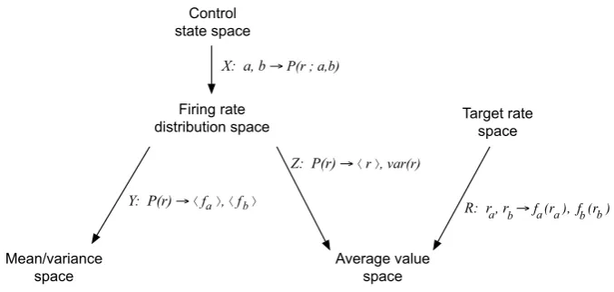
Now we shall consider the general case in which two control variablesaandbevolve according to arbitrary control functions fa and fb and control the distribution of a neuron’s firing rater. We make the dependence of this distribution on a andb
explicit by writing the distribution ofr asP (r;a, b). We address several questions to this model. First, what fixed points exist for a given control system, and what characterizes these fixed points? Second, under what circumstances are these fixed points stable?
In this section, we answer these questions under the simplifying assumption that
fa(r)andfb(r)are constant on any domain whereP (r;a, b) >0. In Appendices1
and2, we show that our results persist qualitatively for nonconstantfaandfb. In Theorem1, we write expressions for the firing rate meanμ∗ and varianceν∗
that characterize any fixed point(a∗, b∗). From this result we find that the difference between the two target firing rates plays a key role in establishing the characteristic variance at a control system fixed point.
In Theorem 2, we present a general condition that ensures that a fixed point
3.1 Definitions
Consider a pair of homeostatic variablesaandbwhose instantaneous rates of change are functions of a firing rate variabler:
τa
a˙=fa(ra)−fa(r), τb
b˙=fb(rb)−fb(r),
(6)
where 0< 1 is a multiplier separating the fast time scale of firing rate variation and the slow time scale of homeostasis,τa andτb are homeostatic time constants (in units of slow time),ra andrb are the target firing rates of the two homeostatic mechanisms, andfa andfbare smooth increasing bounded functions with bounded derivatives. Note that we have introduced the small parameterrepresenting the sepa-ration of the time scales of homeostasis and firing rate dynamics rather than assuming thatτaandτbare large. This form is sufficiently general to encompass a wide range of different feedback strategies.
Remark 1 In order to describe the evolution of a homeostatic variablea that acts multiplicatively and must remain positive (e.g., the synaptic scaling multipliergused in many of our examples), we can instead set τaa˙=a(fa(ra)−fa(r)). We can then put this system into the general form above by replacingawitha˜:=log(a), whose evolution is described by the ODEτaa˙˜=fa(ra)−fa(r).
We assume that, for fixeda andb, the firing rate r(t;a, b)(written as a func-tion of time and control variables) is distribufunc-tion-ergodic with stafunc-tionary firing rate distributionP (r;a, b), that is, limT→∞T10Tf (r(t;a, b)) dt=Rf (r)P (r;a, b) dr
with probability 1 for all integrable functions f. For brevity of notation, we let ·(a,b):=E(·|a, b)denote the expected value of a function of r over the station-ary distributionP (r;a, b)(or, equivalently, the time average of this function over timeT → ∞), given a control system state(a, b). Letμ(a, b)andν(a, b)denote the mean and variance ofP (r;a, b), respectively.
Averaging (6) over the invariant distribution, we arrive at the “averaged equa-tions”:
τa
a˙≈Fa(a, b):=fa(ra)−
fa(r)
(a,b),
τb
b˙≈Fb(a, b):=fb(rb)−
fb(r)
(a,b).
(7)
We use the averaged equations to study the behavior of the unaveraged system (6). Sincermay be constantly fluctuating,aandbmay continue to fluctuate even once a fixed point of the averaged system has been reached, so we cannot expect stable fixed points in the classical sense. Instead, we define a weaker form of stability.
at(a∗, b∗)for all time with probability 1. Intuitively, a point is stable in the small-
limit if trajectories become trapped in a ball around that point, and the ball is smaller when homeostasis is slower.
Lemma 1 Any exponentially stable fixed point of the averaged system (7) is a stable fixed point of the original system (6) in the small-limit.
Proof This follows from Theorem 10.5 in [15].
3.2 Main Results
3.2.1 Fixed Points
Given a homeostatic control state(a∗, b∗), it is straightforward to find the target firing rates that make that state a fixed point in terms of the average values of
fa andfb. By setting a˙= ˙b=0 in (7) we find that ra=fa−1(fa(r)(a∗,b∗))and
rb=fb−1(fb(r)(a∗,b∗)). (These expressions are well defined becausefa is increas-ing and hence invertible, andfa(r)(a∗,b∗)must fall within the range offa; likewise forb.)
Given a pair of target firing ratesraandrb and functionsfaandfb, we can ask what states(a∗, b∗)become fixed points of the averaged system. We shall answer this question in order to show that (1) whenfaandfbare constant, the fixed points are exactly the points at whichP (r;a, b)attains a certain characteristic mean and variance, (2) the relative convexities of the control functions determine whetherraor
rbmust be larger for fixed points to exist, and (3) fixed points with high firing rate variance are achieved by settingrbfar fromra.
Theorem 1 Consider a dual control system as described in Sect. 3.1with target firing ratesraandrband control functionsfaandfb. LetKa:=f
a(ra) fa(ra),Kb:=
fb(rb) fb(rb), andk:= Ka−KbKa−Ka+KbKb(rb−ra). We consider a domain of control system states(a, b)
on which each distributionP (r;a, b)has constantfa(r)andfb(r)on its support. The fixed points of the averaged control system in this domain are exactly the points
(a∗, b∗)at which the meanμ(a∗, b∗)isμ∗ and the varianceν(a∗, b∗)isν∗, where we define
μ∗:=ra+rb
2 +
rb−ra 2 k,
ν∗:= rb−ra Kb−Ka
2−rb−ra 4
(Kb−Ka)
1+k2−2(Ka+Kb)k .
We will henceforth callμ∗andν∗the “characteristic” mean and variance of any neuron regulated by this control system.
Remark 3 In Appendix1, we show that this result persists in some sense for noncon-stantfaandfb. Specifically, if variation infaandfbover the appropriate domain is small, the mean and variance at any fixed point are close toμ∗andν∗, and every point at which the mean isμ∗and the variance isν∗is close to a fixed point.
Proof We abbreviateμ(a, b)as μandν(a, b)asν. Sincefa andfb have constant second derivatives on the domain of interest, we can write
fa(r)=fa(ra)+fa(ra)(r−ra)+ 1 2f
a(ra)(r−ra)2. Taking the expected values of both sides, we have
fa(r)
(a,b)=fa(ra)+fa(ra)(μ−ra)+ 1 2f
a(ra)
(r−ra)2
(a,b).
A simple calculation gives us(r−ra)2(a,b)=ν+(μ−ra)2, so we can write
fa(r)
(a,b)=fa(ra)+fa(ra)(μ−ra)+ 1 2f
a(ra)ν+ 1 2f
a(ra)(μ−ra)2. At a fixed point(a∗, b∗)of the averaged control system with firing rate meanμ∗and varianceν∗, we have 0= ˙a=fa(ra)− fa(r)(a∗,b∗), or
0=fa(ra)
μ∗−ra
+1 2f
a(ra)ν∗+ 1 2f
a(ra)
μ∗−ra 2
,
0=Kaν∗+2
μ∗−ra
+Ka
μ∗−ra 2
.
(8)
Deriving a similar expression by expandingfb(r)aroundrb, we have
0=Kbν∗+2
μ∗−rb
+Kb
μ∗−rb 2
. (9)
Multiplying (8) byKband (9) byKaand taking the difference, theν∗terms cancel, leaving
0=2Kb
μ∗−ra
−2Ka
μ∗−rb
+KaKb
μ∗−ra 2
−KaKb
μ∗−rb 2
.
Solving forμ∗, we have
μ∗=2Karb−2Kbra+KaKb(ra−rb)(ra+rb)
2(Ka−Kb)+2KaKb(ra−rb)
or
μ∗=ra+rb
2 +
rb−ra 2
Ka+Kb
Ka−Kb−KaKb(rb−ra)
=ra+rb
2 +
wherek=Ka−KbKa−KaKb+Kb(rb−ra). Taking the difference of (8) and (9), we get
0=(Ka−Kb)ν∗+2(rb−ra)+Ka
μ∗−ra 2
−Kb
μ∗−rb 2
or, substituting forμ∗and solving forν∗,
ν∗=(rb−ra) Kb−Ka
2−rb−ra 4
(Kb−Ka)
1+k2−2(Ka+Kb)k .
Given the parameters of the control system (including a pair of target firing rates), this theorem shows that achieving a specific firing rate mean and variance is necessary and sufficient for the time-averaged control system to reach a fixed point. IfP (r;a, b)
(the distribution of the firing rate as a function ofa andb) changes, as it might as a result of changes in the statistics of neuronal input, then the new fixed points will be the new points at which this firing rate mean and variance are achieved. Conversely, given a desirable firing rate mean and variance, we could tune the parameters of the control system to make these the characteristic mean and variance of the neuron at control system fixed points.
Whether any fixed point(a∗, b∗)actually exists depends on whether the charac-teristic firing rate mean and variance demanded by Theorem1can be achieved by the neuron, that is, fall within the range ofμ(a∗, b∗)andν(a∗, b∗). If the mapping from
(a, b)to(μ, ν)is not degenerate, then there exists a nondegenerate (two-parameter) set of reachable values ofμandνfor which control system fixed points exist. In the degenerate case that neitherμnorν depend onb, the set of reachable values of μ
andν are a degenerate one-parameter family in a two-dimensional space. This cor-responds to the case of a single-mechanism control system. In this case, a control system possesses a fixed point with a given firing rate mean and variance only if they are chosen in a particular relationship to each other. A perturbation to neuronal pa-rameters would displace this one-parameter family in the(μ, ν)-space, likely making the preperturbation firing rate mean and variance unrecoverable.
We now prove a corollary giving a simpler form of Theorem1, which holds if
rb−rais sufficiently small.
Corollary 1 GivenKa and Kb, let K=max(|Ka|,|Kb|). Ifra andrb are chosen such thatK|rb−ra|and K
2
|Kb−Ka||rb−ra|are sufficiently small, then the characteristic mean and variance given in Theorem1are arbitrarily well approximated by
μ∗≈ra+rb
2 −
rb−ra 2
Ka+Kb
Kb−Ka
,
ν∗≈2 rb−ra
Kb−Ka
.
Proof Forkdefined in Theorem1, we can write
k= Ka+Kb (Ka−Kb)(1−KaKa−KKb
b(rb−ra))
so that if |KK2
b−Ka||rb−ra|is sufficiently small, thenkis arbitrarily close to Ka+Kb Ka−Kb. This gives us an approximation ofμ∗. We can also use it to write
rb−ra
4
(Kb−Ka)
1+k2−2(Ka+Kb)k
≈1 4
(Kb−Ka)(rb−ra)+
Ka2+2KaKb+Kb2
Ka−Kb
(rb−ra)
−2K
2
a+2KaKb+Kb2
Ka−Kb
(rb−ra) .
All of these terms are bounded in norm by multiples of either K|rb −ra| or K2
|Kb−Ka||rb−ra|, so this expression is arbitrarily small. This gives us an
approxi-mation forν∗.
The range ofrb−rafor which this result holds is determined byKaandKb, mea-sures of the convexities of the control functions. Informally, we say that this corollary holds ifrb−rais “small on the scale of the convexity of the control functions.”
From the corollary we draw two important conclusions that hold whilerb−ra remains small on the scale of the convexity of the control functions:
1. Since a negative firing rate variance can never be achieved by the control system, there can only be a fixed point ifrb−raandKb−Katake the same sign. 2. Increasing|rb−ra|causes a proportionate increase in control system’s
character-istic firing rate variance.
3.2.2 Fixed Point Stability
Next, we address the question of whether a fixed point of the averaged control system is stable. We again make the simplifying assumption thatfaandfbare constant and then drop this assumption in Appendix2.
Theorem 2 Let(a∗, b∗)denote a fixed point of the averaged control system described above. We assume the following:
1. The functionsμandνare differentiable at(a∗, b∗). 2. ∂Fa∂a and∂Fb
∂b are negative at(a∗, b∗), that is, on average,aandbprovide negative feedback tornear(a∗, b∗).
3. For(a, b)in a neighborhood of(a∗, b∗),faandfbare constant on any domain ofrwhereP (r;a, b) >0.
Letμ∗=μ(a∗, b∗)andν∗=ν(a∗, b∗)denote the firing rate mean and variance at this fixed point. Below, all derivatives ofμ and ν with respect toa and b are evaluated at(a∗, b∗).
The fixed point(a∗, b∗)of the averaged system is stable if
∂μ ∂a
∂ν ∂b −
∂μ ∂b
∂ν ∂a
fb(μ∗) fb(μ∗) −
fa(μ∗)
Remark 4 Note that this result isa/b symmetric: ifa andb are swapped, then the signs of both terms reverse and these sign changes cancel, leaving the stability con-dition unchanged.
Proof A fixed point(a∗, b∗) of the averaged system is exponentially stable if the Jacobian
J=
∂Fa ∂a
∂Fa ∂b ∂Fb
∂a ∂Fb
∂b
evaluated at (a∗, b∗) has two negative eigenvalues. By Assumption 2, the Jaco-bian of the dual control system at (a∗, b∗)has negative trace. A matrix has two negative eigenvalues if it has a negative trace and positive determinant. There-fore, the fixed point(a∗, b∗)of the averaged control system is exponentially stable if
det(J )=∂Fa ∂a
∂Fb
∂b − ∂Fa
∂b ∂Fb
∂a >0
at(a∗, b∗).
Below, we abbreviateμ(a, b)as μandν(a, b)asν. In order to write useful ex-pressions for the terms in det(J ), we Taylor-expand fa(r) aboutμ out to second order, writingfa(r)=fa(μ)+fa(μ)(r−μ)+
r
μ(r−s)fa(s) ds. We similarly ex-pandfb(r)and average these expressions at (a, b)to rewrite the averaged control equations:
Fa(a, b)=fa(ra)−fa(μ)−
r
μ
(r−s)fa(s) ds
(a,b)
,
Fb(a, b)=fb(rb)−fb(μ)−
r
μ
(r−s)fb(s) ds
(a,b)
.
Differentiating these expressions and evaluating them at(a∗, b∗), we calculate the terms in det(J ):
∂Fa
∂b = − ∂μ ∂bf
a
μ∗− ∂ ∂b
r
μ
(r−s)fa(s) ds
(a,b)
, (11)
where all derivatives are evaluated at(a∗, b∗). We have assumed thatfa(r)≡fa(μ∗)
over the support ofP(a∗,b∗), so we can write
∂Fa
∂b = − ∂μ ∂bf
a
μ∗−faμ∗ ∂ ∂b
r
μ
(r−s) ds
(a,b)
= −∂μ
∂bf
a
μ∗−1
2f
a
Likewise for the other three terms∂Fa∂a, ∂Fb∂a, and ∂Fb∂b. Calculating the determinant ofJ and canceling like terms, we have
det(J )=1
2 ∂μ ∂af a
μ∗fbμ∗∂ν ∂b− 1 2 ∂μ ∂bf a
μ∗fbμ∗∂ν ∂a +1 2 ∂μ ∂bf b
μ∗faμ∗∂ν ∂a − 1 2 ∂μ ∂af b
μ∗faμ∗∂ν
∂b (12) =1 2 ∂μ ∂a ∂ν ∂b − ∂μ ∂b ∂ν ∂a f a
μ∗fbμ∗−fbμ∗faμ∗. (13)
Thus,(a∗, b∗)is exponentially stable if
0<1
2 ∂μ ∂a ∂ν ∂b − ∂μ ∂b ∂ν ∂a f a
μ∗fbμ∗−fbμ∗faμ∗
or, equivalently, if
0< ∂μ ∂a ∂ν ∂b − ∂μ ∂b ∂ν ∂a
fb(μ∗) fb(μ∗)−
fa(μ∗)
fa(μ∗) .
Remark 5 In Appendix2, we drop the assumption thatfaandfbare constant over the range ofrand derive a sufficient condition for stability of the form
∂μ ∂a ∂ν ∂b − ∂μ ∂b ∂ν ∂a
fb(μ∗) fb(μ∗) −
fa(μ∗)
fa(μ∗) > Δ (14)
for aΔ≥0 that is close to zero iffaandfbdo not vary too widely over most of the range ofr.
Remark 6 A similar result to Theorem2could be proven for a system with a single slow homeostatic feedback. The limitation of such a system would be in reachability. As the single homeostatic variableachanged, the firing rate meanμand varianceν
could reach only a one-parameter family of values in the(μ, ν)-space. Thus, most mean/variance pairs would be unreachable. A perturbation to neuronal parameters would displace this one-parameter family in the(μ, ν)-space, likely making the orig-inal mean/variance pair unreachable. Thus, a single homeostatic feedback could only succeed in recovering its original firing rate mean and variance after perturbation in special cases.
By Lemma1, fixed points of the averaged system that satisfy the criteria for sta-bility under Theorem2are stable in the small-limit for the full, un-averaged control system.
4 Further Single-Cell Examples
We will focus on examples in which the two homeostatic variables are excitabilityx
The generality of the main results above (which require thatfa andfbbe con-stant) allows us to investigate a range of different models of firing rate dynamics even if we do not have an explicit expression for the rate distributionP. We only need to know dependence of the firing rate meanμand varianceν on the control variables to use Theorem1to identify control system fixed points and to use Theorem 2to determine whether those fixed points are stable.
In the more general case addressed in Appendix2, where the second derivatives are not assumed to be constant, the left side of (10) must be positive and sufficiently large to guarantee the existence of a stable fixed point, where the lower boundΔ
for “sufficiently large” is close to zero iffa andfb are nearly constant over most of the distribution P (r;a, b). We will further discuss the simpler case, but all of our analysis can be applied to the more general case by replacing “positive” with “sufficiently large.”
Returning to Example1 We can use Theorem2to generalize the results for the dually controlled OU process from Sect.2. We consider the rate model described by the differential equation
τrr˙= −r+gI (t )+x, (15)
whereI (t )is any second-order stationary process, that is, a process with stationary meanφ= I (t ) and stationary autocovariance functionR(w)= I (t )I (t+w) − φ2, both independent oft. We assume thatr is ergodic. Letμ∗ andν∗ denote the characteristic firing rate mean and variance determined from the parameters of the control system parameters using Theorem1.
This firing rate process is the output of a stationary linear filter applied to a second-order stationary process, so according to standard results, we haveμ(x, g)=gφ+x
andν(x, g)=g22τC
r , whereC=
t
−∞R(t1−t2)e−
2t−t1−t2
τr dt1dt2. Thus, as long as
ν∗>0, there exists a fixed point of the control system at
x∗, g∗=
μ∗−
2τrν∗
C φ,
2τrν∗
C .
At this fixed point, we have ∂μ∂x =1, ∂μ∂g =φ, ∂x∂ν =0, and ∂ν∂g =gτr∗C. This gives us
∂ν ∂g
∂μ ∂x −
∂ν ∂x
∂μ
∂g >0, and the conditions for Theorem2are met if fg(μ∗) fg(μ∗) −
fx(μ∗) fx(μ∗) is positive.
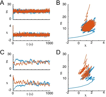
Figure3 shows simulation results for this system under conditions sufficient for stability. Note that if the statistics of the inputI (t )change, the fixed point changes so that the system maintains its characteristic firing rate mean and variance at equilib-rium. In Fig.4A and Fig.4B, we alter this system by increasingand by givingI (t )
correlations on long time scales, respectively. In both these cases, trajectories fluctu-ate widely about the fixed point of the averaged system but remain within a bounded neighborhood, consistent with the idea of stability in the small-limit.
The slopesfgandfx can be understood as measures of the strength of the home-ostatic response to deviations from the target firing rate, and the second derivatives
Fig. 3 Intrinsic/synaptic dual homeostasis recovers original mean and variance after perturbation in a simulated firing rate model. Firing rateris described by equation (15) with parameter values listed in Appendix3. Input current is set toI (t )=φ+σ ξ (t ), whereξ (t )is white noise with unit variance. In the top row of figures,φ=0.5 andσ=0.25; in the bottom row of figures,φ=2.5 andσ=0.75. (A)xand
gtrajectories plotted over time from two different initial conditions (orange and blue) as a fixed point is reached. (B) The same trajectories plotted inx/gphase space. (C) Mean firing rater(above) and firing rate variance var(r)(below) are calculated as a function of homeostatic state(x, g)and represented by color inx/gparameter space. The fixed point is marked in white. (D) Mean firing rater(above) and firing rate variance var(r)(below) are plotted over time for both initial conditions. (E)-(H) When the mean and variance of the input current are increased, the system seeks out a new homeostatic fixed point. Note in G and H that, in spite of the new input statistics, a fixed point is reached with the same firing rate mean and variance
upward and downward rate deflections. Ifx andgare rescaled to setfg≈fx, then Theorem2predicts that dual homeostasis stabilizes a fixed point with a given char-acteristic mean and variance iffg(μ∗) > fx(μ∗), thats is, if the (signed) difference between the effects of positive rate deflections and negative rate deflections is greater for the synaptic mechanism than for the intrinsic mechanism.
Example 2 (Intrinsic noise) In Example1, we assumed that all of the rate fluctuation was due to fluctuating synaptic input. If we introduce an intrinsic source of noise (e.g., channel noise), then the picture becomes slightly more complicated. We set
τrr˙= −r+gI (t )+x+ηξ (t ), (16)
whereξ (t )is unit-variance white noise independent ofI (t ), andηsets the magnitude of the noise. The same calculations as before show that the conditions for stability under Theorem2are met at any fixed point for fg(μ∗)
fg(μ∗) − fx(μ∗)
Fig. 4 Convergence of intrinsic/synaptic dual homeostasis is compromised by short homeostatic time constants and temporally correlated noise. Firing rateris described by equation (15) with parameter val-ues listed in Appendix3. (A)-(B) The system simulated for Fig.1A-D is modified by reducing homeostatic time constants by a factor of 50: we setτx=10 s andτg=1,000 s. Trajectories enter and remain within
a large neighborhood of the fixed point observed in Fig.1A, but fluctuate randomly within that neighbor-hood. By Lemma1these trajectories converge in the small-limit, so this neighborhood represents the ball of radiusα()that traps all trajectories and shrinks to zero as→0. (C)-(D) The system described in Fig.1A is modified by introducing long temporal correlations into the time course of the input current:
I (t )is an Ornstein-Uhlenbeck process described by the SDEτIdI= −I dt+dξ, whereξis white noise
with unit variance andτI=10 s. Again, trajectories enter and remain within a large neighborhood of the
fixed point observed in Fig.1A but fluctuate randomly within that neighborhood
firing rate variance includes the noise variance:ν(x, g)=g22τrC+ 2ητr2. Under Theo-rem1, a fixed point only exists if control system parameters are chosen to establish a characteristic variance ofν∗>2ητr2. This neuron cannot be stabilized with variance less than 2ητ2
r because a variance that low cannot be achieved by the inherently noisy neuron.
In Fig.5, we show the behavior of this system when ν∗> 2ητ2
r (the mean and variance necessary for a fixed point are in the ranges ofμandν) and whenν∗<2ητr2
(the necessary variance is not in the range ofν).
in-Fig. 5 Dual homeostasis tolerates some intrinsic firing rate noise but fails to converge if noise is suffi-ciently strong. The dynamics of the firing raterare modeled by an intrinsically noisy OU process described by equation (16) with parameter values listed in Appendix3. (A) Intrinsic noise amplitude is set toη=2. Dual homeostasis converges on a fixed point near the fixed point of the corresponding system with no intrinsic noise, illustrated in Fig.1A-D. (B) Firing rate meanrand variance var(r)are calculated and displayed as functions ofx andginx/g parameter space. The fixed point of the system is marked in white. (C) Intrinsic noise amplitude is set toη=10. Dual homeostasis fails to converge:xwinds up with-out bound, andgwinds down toward zero. (D) Note that, due to intrinsic noise, the firing rate variance everywhere in parameter space is larger than the characteristic variance reached at equilibrium in B. Thus, the characteristic variance of this system at equilibrium is unreachable, and dual homeostasis does not converge
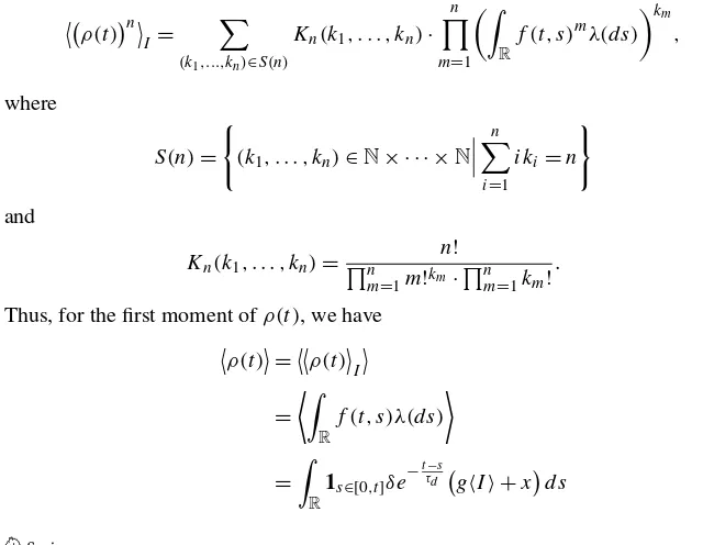
crease instantaneously byδat each spike and decay exponentially with time constant
τdbetween spikes. We assume thatρis ergodic.
We show in Appendix4 that, after sufficient time,y =ρ assumes a stationary distribution with meanμ(x, g)=δτd(gφ+x)and varianceν(x, g)=δ2τd(Cg2+
gφ+x
2 ), where φ is the stationary mean of I (t ), and C is a positive constant
de-termined by the stationary autocovariance of I (t ). Thus, we calculate ∂x∂ν = δ2τd
2 ,
∂μ
∂g =δτdφ, ∂ν
∂g=2δ2τdCg∗− δ2τ
dφ
2 , and
∂μ
∂x =δτd, and we find that ∂ν ∂g
∂μ ∂x−
∂ν ∂x
∂μ ∂g = 2δ3τd2Cg∗>0. As in Examples1and2, we conclude that the conditions for stability under Theorem2are met if fg(μ∗)
fg(μ∗) − fx(μ∗) fx(μ∗) >0.
Note that the conditions for stability in this model are the same as the conditions in the firing rate models. In [8], we show the same result empirically for biophysically detailed model neurons. What all these models have in common is that changes ing
mainly the firing rate mean and has little or no effect on the variance. These results suggest that fg(μ∗)
fg(μ∗) − fx(μ∗)
fx(μ∗) >0 is a general, model-independent condition for sta-bility of synaptic/intrinsic dual homeostasis. In Appendix2, where control function second derivatives are not assumed to be constant, this condition is replaced by the condition of sufficiently largefg(μ∗)
fg(μ∗) − fx(μ∗) fx(μ∗).
As in Example2, not all mean/variance pairs can be achieved by the control sys-tem: no matter how smallgis, we still haveν(x, g)≥δ2τgφ2+x =δμ(x,g)2 due to the inherently noisy nature of Poisson spiking, which acts as a restriction on the range ofν. We also must haver >0, so the range of μis constrained toμ(x, g) >0. If
rxandrgare chosen such that the characteristic firing rate meanμ∗and varianceν∗ defined in Theorem1obey these inequalities, then there exists a control system state
(x∗, g∗)at which Theorem1is satisfied and which is therefore a fixed point.
5 Recurrent Networks and Integration
A recurrent excitatory network has been shown to operate as an integrator when neu-ronal excitability and connection strength are appropriately tuned [9, 10]. Such a network can maintain a range of different firing rates indefinitely by providing exci-tatory feedback that perfectly counteracts the natural decay of the population firing rate. When input causes the network to transition from one level of activity to an-other, the firing rate of the network represents the cumulative effect of this input over history. Thus, the input is “integrated.”
Below, we show that the parameter values that make such a network an integrator can be stably maintained through dual homeostasis as described before. Importantly, we also show that an integrator network made stable by dual homeostasis is robust to variations in control system parameters and (as in the previous examples) unaffected by changes in input mean and variance. In this section, we build intuition for this phe-nomenon by investigating a simple example network consisting of one self-excitatory firing rate unit, which may be taken to represent the activity of a homogeneous recur-rent network. In Appendix5, we perform similar analysis forN rate-model neurons with heterogeneous parameters. In this case, we do not prove stability, but we do demonstrate that if any neuron’s characteristic variance is sufficiently high, then the network is arbitrarily close to an integrator at any fixed point of the control system.
We consider a single firing rate unit described by the equation
˙
r= −r+gr+I (t )+x+ηξ (t ),
whereηis the level of intrinsic noise,I (t )is a second-order stationary synaptic input with meanφand autocovarianceR(w), andξ (t )is a white noise process with unit variance. (For simplicity, we have rescaled time to set the time constantτr to 1.) Let
m(t )denote the expected value of r at timet. Taking the expected values of both sides of the equation, we have
˙
Letμdenote the expected value ofr once it has reached a stationary distribution. Settingm˙ =0, we calculate
μ=gφ+x
1−g . (17)
Lets(t )denote the deviation ofr from mat timet:s(t ):=r(t )−m(t ). From the equations above we have
˙
s= −s+gs+I (t )−φ+ηξ (t ). (18)
If we setg=1, then thes-dependence drops out of the right side, and we have
s(T )=s(0)+
T
t=0
I (t )−φ+ηξ (t )dt.
In this extreme case,sacts as a perfect integrator of its noise and its input fluctuations, that is, as a noisy integrator. Forgclose to 1, the mean-reversion tendency of s is weak, so on short time scales,sacts like a noisy integrator.
Next, we write a differential equation for the variance ofr. From (18) we write
s(t+dt )=s(t )+dt−s(t )+gs(t )+I (t )−φ+ηξ (t ).
Squaring both sides out toO(dt )and taking the expected value, we have
s(t+dt )2=s(t )2−2s(t )2(1−g) dt+g2C dt+η2dt,
whereC is a positive constant depending onτr and R(w)as in the previous sec-tion. Letν:=limt→∞var(r(t ))=limt→∞s(t )2denote the expected variance ofr
when it has reached a stationary distribution. At this stationary distribution, we have s(t+dt )2 = s(t )2, so
0= −2(1−g)ν+g2C+η2
or
ν=1
2
g2C+η2
1−g . (19)
This relation betweengandν is plotted in Fig.6. The right side of this equation is η22 atg=0 and increases withguntil it asymptotes to infinity atg=1. So, given
Fig. 6 Firing rate varianceνvs. synaptic strengthgin an excitatory recurrent network. Equation (19) is plotted withη2=5 andC=1. When synaptic strength is zero, all firing rate variance is due to noise, soν=η22. As synaptic strength increases, firing rate variance increases. As synaptic strength approaches unity, recurrent excitation acts to reinforce variations in firing rate, and variance asymptotes to∞. If target firing rates are set such that the characteristic firing rate varianceν∗is large, then the synaptic strengthg∗
at a control system fixed point must be close to unity, making the network an integrator of its inputs
in this way is robust to variation in characteristic variance ν∗ (and unaffected by variation inμ∗).
We can use (17) and (19) to calculate
∂ν ∂g
∂μ ∂x −
∂ν ∂x
∂μ ∂g =
gC
1−g+ η2
2(1−g)2 >0,
so as in the previous examples, the conditions for Theorem2are met, and stability of
any fixed point is guaranteed ifffgg(μ(μ∗∗))− fx(μ∗) fx(μ∗) >0. In short, iffg(μ∗)
fg(μ∗) − fx(μ∗)
fx(μ∗) >0 and target rates are chosen to create a sufficiently large characteristic varianceν∗, then dual homeostasis of intrinsic excitability and synaptic strength stabilizes a recurrent excitatory network in a state such that the net-work mean firing rate acts as a near-perfect integrator of inputs shared by the popula-tion. The corollary to Theorem1tells us that, to first approximation, the characteristic variance is proportionate to the difference between the target rates, and a large char-acteristic variance is achieved by setting the homeostatic target rates far apart from each other. The integration behavior created in this way is robust to variation in the characteristic mean and variance, and therefore robust to the choice of target firing rates.
of the firing rate is effectively infinite.) Thus, the network can attain a large variance by tuningg to be sufficiently close to 1. If this large variance is the characteristic variance of the control system, then there is a fixed point of the dual control system at this value ofg.
In some sense, this behavior is an artifact of the model used—perfect integration is only possible if the feedback perfectly counters the decay of the firing rate over a range of different rates, which is possible in this model because rate increases linearly with feedback and feedback increases linearly with rate. However, such a balance is also achievable with nonlinear rate/feedback relationships if they are locally linear over the relevant range of firing rates. In particular, if the firing rate is a sigmoidal function of input and the eigenvalue of firing rate dynamics near a fixed point is near zero, the upper and lower rate limits act to control runaway firing rates while the system acts as an integrator in the neighborhood of the fixed point. In [8], we show that a recurrent network of biophysically detailed neurons with sigmoidal activation curves can be robustly tuned by dual homeostasis to act as an integrator.
In Appendix5, we show that integration behavior also occurs at set points in net-works of heterogeneous dually homeostatic neurons if one or more of them have a sufficiently large characteristic variance. If only one neuron’s characteristic variance is large, the afferent synapse strength to that neuron grows until that neuron gives itself enough feedback to act as a single-neuron integrator as described before. But if many characteristic variances are large, then all synapse strengths remain biophys-ically reasonable, and many neurons participate in integration, as might be expected in a true biological integrator network.
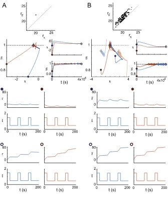
In Fig.7, we show simulation results for homogeneous and heterogeneous re-current networks with target firing rates set to create sufficiently large characteristic firing rate variances. In addition to corroborating our analytical results, these simu-lations provide empirical evidence that the fixed points of heterogeneous networks are stable under similar conditions to those guaranteeing the stability of the single self-excitatory rate unit discussed before.
6 Discussion
This mathematical work is motivated by the observation that the mean firing rates of neurons are restored after chronic changes in input statistics and that this firing rate regulation is mediated by multiple slow biophysical changes [3,5]. We explore the possibility that these changes represent the action of multiple independent slow neg-ative feedback (“homeostatic”) mechanisms, each with its own constant “target firing rate” at which it reaches equilibrium. Specifically, we focus on a model in which the firing of an unspecified model neuron is regulated by two slow homeostatic feed-backs, which may correspond to afferent synapse strength and intrinsic excitability or any two other neuronal parameters.
Fig. 7 Dual homeostasis creates integrators from a single recurrently excitatory neuron and a heteroge-neous excitatory network. (A) Dual homeostasis tunes a single neuron with a recurrent excitatory con-nection to function as an integrator from two different initial conditions (orange and blue). First row: the target ratesrxandrgare plotted as a point in(rx, rg)space. Second row: the resultingxandgtrajectories
are plotted in phase space and over time. Third row: before dual homeostasis, the neuron is tested for inte-grator-like behavior by injecting pulsatile inputI (t ). The firing raterreturns to a baseline after each pulse. Fourth row: after dual homeostasis, firing raterincreases at each pulse and retains its approximate value from one pulse to the next. This neuron is an integrator: its firing rate at any time represents an integral of the pulse history. (B) Analogous plots for a heterogeneous recurrently excitatory network of 200 neurons initialized from two initial conditions (orange and blue). Top row: target firing rate pairs of all neurons are plotted in(rx, rg)space. Note thatrgis always chosen to be greater thanrx. Second row: average values
such dual homeostasis to exhibit this behavior. Importantly, the homeostatic system reaches a fixed point when the firing rate mean and variance reach characteristic values determined by homeostasis parameters, so the mean and variance at equilib-rium are independent of the details of the neuron model, including stimulus statistics. Thus, this effect can restore a characteristic firing rate mean after major changes in the neuron’s stimulus statistics, as has been observed in vivo, while at the same time restoring a characteristic firing rate variance.
In Theorem1, we have provided expressions for the characteristic firing rate mean and variance established by a specific set of homeostatic parameters. They show that when the separation between the target ratesra andrb is appropriately small, the relative convexities of the functionsfa and fb (by which the firing rate exerts its influence on the homeostatic variables) determine which target rate must be larger for a fixed point to exist. When a fixed point does exist, the characteristic firing rate variance at the fixed point is proportional to the difference betweenrbandra.
In Theorem2, we find that any fixed point of our dual homeostatic control system is stable if a specific expression is positive. This expression reflects the mutual influ-ences of firing rate on the homeostatic control system and of control system on the firing rate mean and variance.
Both these theorems are proven under the simplifying assumption thatfaandfb
are constant. However, in Appendices1and2, we drop this assumption and find that qualitatively similar results hold as long as these second derivatives do not vary too widely. In particular, stability is guaranteed if the expression in Theorem2exceeds a certain positive bound that is close to zero iffaandfbare nearly constant across most of the range of variation of the firing rate.
We have explored the implications of our results for a system with slow homeo-static regulation of intrinsic neuronal “excitability”x (an additive horizontal shift in the firing rate curve) and afferent synapse strengthg. From the corollary to Theorem1
we find that (to first approximation) stable firing rate regulation requiresrg> rx. Using Theorem2, we show that for rate-based neuron models and Poisson-spiking models, stable firing rate regulation is achieved when thefgis sufficiently concave-up relative tofx.
We predict that these conditions on relative concavity and relative target firing rates should be met by any neuron with independent intrinsic and synaptic mecha-nisms as its primary sources of homeostatic regulation. Experimental verification of these conditions would suggest that our analysis accurately describes the interaction of a pair of homeostatic mechanisms; experimental contradiction of these conditions would suggest that the control process regulating the neuron could not be accurately described by two independent homeostatic mechanisms providing simple negative feedback to firing rate.