ORIGINAL PAPER
Effectiveness of link and path information on simultaneous
adjustment of dynamic O-D demand matrix
Ernesto Cipriani&Marialisa Nigro&Gaetano Fusco& Chiara Colombaroni
Received: 25 November 2011 / Accepted: 30 July 2013 / Published online: 15 September 2013
#The Author(s) 2013. This article is published with open access at SpringerLink.com
Abstract
IntroductionThe paper deals with the adjustment of time-dependent Origin–destination (O-D) demand matrix, which is the fundamental input of ITS application for traffic predic-tions. The usual problem is to search for temporal O-D matri-ces that are“near”an a priori estimate (seed matrices) and that best fit traffic counts. However information on link flows is not fully effective in describing the state of the network; recent technologies for tracking vehicles provide a new kind of information on route travel times that can integrate usual information on traffic flows at count sections.
Objective The object of the paper is to analyse the effective-ness of different types of information in the off-line simulta-neous adjustment of dynamic O-D demand, starting from seed matrices with different degrees of reliability.
Keywords Demand adjustment . Dynamic assignment . Probe data . SPSA algorithm
1 Introduction
Dynamic estimation of Origin–destination (O-D) matrix is a fundamental input for ITS systems, which need to identify the current traffic state and predict future traffic conditions at real-time level. In fact, demand patterns vary from day to day and
congested networks are heavily affected by even small changes of O-D demand flows. So, high level of accuracy on demand can lead to successful ITS systems [1] as well as to effective strategies for implementing route guidance, congestion pricing and network-based traffic signal control [2]. On the other hand, knowledge of space-temporal structure of demand is the nec-essary input for a dynamic traffic assignment model that simu-lates congestion evolution. Without correcting errors in O-D demand estimation, the inconsistency in O-D flows would accumulate and propagate in the traffic simulation process, making the network state estimation and prediction highly unreliable [3].
Usual methods for O-D estimation combine some a priori information, like historical O-D matrices, with real-time traffic measurements. Since dynamic traffic assignment models for ITS applications require a very detailed representation of O-D matrix in time and space, the O-D estimation problem is highly undetermined. So, any possible information on demand struc-ture can be useful to reduce the complexity of the problem.
Information on prior O-D matrices (the so-called “seed matrix”) are usually reported in any formulation, both static and dynamic; however, differently from other measures, they are not directly observable [4] and solution procedures for demand adjustment are usually irrespective of their quality [5]. Current technologies can provide a great amount of traffic data collected on links and nodes of the transportation net-work: pavement-embedded sensors, roadside radars and cam-eras provide measures of flows and speeds at nodes and along links; Advanced Vehicle Identification (AVI), ground-based radio navigation, cellular geo-location and GPS provide a new kind of information about travel times and route choices that integrate usual information on traffic flows at count sections. Moreover, it is well known that traffic counts are not fully effective in discerning between congested and uncongested traffic state of a link, because of non-monotone flow-density relationship. Thus, it is important to formulate effective methods for O-D estimation combining several heterogeneous
Electronic supplementary materialThe online version of this article (doi:10.1007/s12544-013-0115-z) contains supplementary material, which is available to authorized users.
E. Cipriani
:
M. Nigro (*)Department of Engineering, Roma Tre University, Via Vito Volterra 62, 00146 Rome, Italy e-mail: [email protected]
G. Fusco
:
C. Colombaronisources of information and to assess the relative importance of each of them. On the other hand, optimization methods can applied to individuate the best locations of measurement sec-tions (see, for example, [6]).
Many authors dealt with the problem of increasing the amount of information required by dynamic O-D estimation problem and included, for example, speed and link occupancy [7–9], probe data from vehicle equipped by AVI tags [10–14,
15,16], aggregate demand data such as traffic emissions and attractions by zones [8,9,17], total demand for sub-networks, or the temporal distribution of trips in some areas on the network. In this paper we want to investigate the contribution of different kinds of information to improve the accuracy of time-dependent O-D matrix estimation. Specifically, with re-spect to previous studies, we introduce information on travel times, which are assumed to be provided by a fleet of floating cars. In order to focus on basic issues of the problem, we tackle off-line simultaneous estimation of time-dependent O-D demand, which is the basis for a suitable development of ITS applications in on-line context.
The paper is organized into five sections including this introduction: Section2reports different methodologies devel-oped in the last years for the dynamic OD estimation and after defines the one adopted in the study; in Section3 the case study is presented, while the results of the application are reported in Section4; finally Section5summarizes the main conclusions.
2 Problem formulation
Different approaches and solution algorithms have been de-veloped in the last years for both off-line and on-line dynamic OD estimation: in the following the most recent contributes are reported.
Zhou et al. [18] formulated the dynamic OD estimation problem as a single level nonlinear optimization model, solved with a relaxation algorithm of the lagrangian extension of the original one, taking into account route choice in order to work in the path- flow dimension. Frederix et al. [23] adopted a linear approximation of the relationship between O-D flows and link flows, taking into account link flows being not separable. This approximation has been obtained with the marginal computation (MaC) method that performs a pertur-bation analysis in a computationally efficient way, using the kinematic wave theory principles for traffic simulation. Tole-do and Kolechkina [19] proposed a method based on a linear approximation of the assignment matrix; they apply different iterative algorithms, performing a mesoscopic traffic simula-tion to conduct network loadings. Djukic et al. [20] proposed the reduction and approximation of OD demand variables based on principal component analysis (PCA). The new transformed set of variables (demand principal components)
is then updated online from traffic counts in a novel reduced state space model for real time estimation of OD demand.
The problem of off-line simultaneous estimation of tempo-ral O-D matrices is tackled in this paper adopting a simulation approach, which avoids introducing assignment matrices [9]. The O-D estimation problem is formulated as an optimization problem aiming at minimizing a linear combination of the distance between estimated and a priori O-D demand flows and the errors between detected and estimated traffic measure-ments in a dynamic (i.e., time-dependent) off-line context. The objective function includes different kinds of data col-lected with different types of techniques: simple traffic counts and speed measurements detected at fixed road sections and travel times measured on routes travelled, for example, by floating cars equipped with a GPS receiver and a cellular mobile transmitter. Adding speed measurement provides fur-ther information on the traffic regime that enables to distin-guish between congested and uncongested conditions. The extent of such a congested condition can be grasped further by adding travel time information.
Given:
a networkB=[N,A], where:
N nodes
A directed links
nod number of origin–destination pairs R routes connecting each OD pair.
the period of analysisT, divided intonhintervals, a subset of linksS={1..ns}∈Aand nodesP={1..np}∈Nequipped with sensors, a subset of monitored routes ρ={1..nr}∈ R, the problem is formulated as it follows:
d1…dnh
¼argminx
1…xnh
ð Þ
fd ðx1…xnn;d1…dnnÞ þ
X
l
fl y1…ynh;by1…bynh
þ
þX
t
ft z1…znh;bz1…bznh
þ
þX
p
fp w1…wnh;wb1…wbnh
2 6 6 6 6 6 6 6 6 4 3 7 7 7 7 7 7 7 7 5
ð1Þ
where:
fd term of the objective function relative to the distance with the seed matrix
xi estimated matrix for departing time intervali, i=1…nh di seed matrix for departing time intervali, i=1…nh yi simulated information on link setSfor departing time
intervali, i=1…nh b
yi collected measures on link setSfor departing time intervali, i=1…nh
fl term of the objective function relative to measures collected on links
bzi collected measures on node setPfor departing time intervali, i=1…nh
fn term of the objective function relative to measures collected on nodes
wi simulated information on route setrfor departing time intervali, i=1…nh
b
wi collected measures on route setrfor departing time intervali, i=1…nh
fp term of the objective function relative to measures collected on routes.
Dependence between simulated information in Eq. (1) and estimated matrices is obtained directly by simulation performing a dynamic traffic assignment (DTA), so that:
y1…ynh ¼ Fðx1…xnhÞ ∀ l z1…znh¼ Fðx1…xnhÞ ∀ t w1…wnh¼Fðx1…xnhÞ ∀ p
ð2Þ
with F=DTA.
Lower bound and upper bound constraints can be intro-duced on demand to avoid infeasible solutions and to restrict the search space:
x1…xnh
ð Þ≥ x1L:B:…xnhL:B:
x1…xnh
ð Þ≤ x1U:B:…xnhU:B:
ð3Þ
Other aggregate demand data can be introduced in the objective function or as a constraint. For example, Cipriani et al. [9] introduce constraints on traffic emissions by zones in order to prevent demand overestimation:
X
i¼1 nh
Goi≤Go ∀o∈foriginsg ð4Þ
with:
Go* a priori emission value for origin zoneo
Goi emission value for origin zoneoof the demand matrix xi.
In fact, overestimation of demand can produce a prolonged loading period in simulation (i.e., the network takes longer to
clear), without significant changes in observed link flows or in the corresponding terms of the objective function. The con-straint on generation balances for the insensitivity of the objective function to these conditions.
Functionsfdepend on the particular estimation framework, on the type of estimator and on the available information [21]. Generalized Least Squares (GLS) framework exploits ad-ditional information about the reliability of measurements; this information can be incorporated as a set of internal weights resulting in the variance–covariance matrix. In such a case, the fdfunction, for instance, assumes the following form:
fdðx1…xnh;d1…dnhÞ ¼ðx−dÞV−1ðx−dÞ ð5Þ
whereV=variance–covariance matrix of the vector of sam-pling errors affecting the estimated.
If this information is not available, the different objective function terms can be controlled using exogenous scalar weights representing the relative confidence of the analyst on measurements (that is: speeds, flows and travel times) or on a priori direct observation (that is, the seed matrix).
Information such as flows and speeds measured on links as well as travel times from probe vehicles has been reported in this study inside the objective function (1). Data from links and routes are considered with different types of grouping to assess the impact of different network elements in the adjust-ment process. Generated trips have been reported as an in-equality constraint as in Eq. (4). Different seed matrices with different degrees of reliability have been considered as inputs of the procedure in order to analyze different levels of uncer-tainty on a priori demand estimation.
The procedure adopted to solve the problem (1) is the SPSA AD-PI (Simultaneous Perturbation Stochastic Approx-imation, Asymmetric Design, Polynomial Interpolation) pro-posed by Cipriani et al. [8]. SPSA AD-PI is a modification of the gradient based path search optimization method that per-mits to reduce the computational effort in regard to the usual gradient-based methods, which is a basic issue to deal with a simultaneous estimation of demand for real applications.
At the generic iteration k, the algorithm computes the dynamic matrix for the next iterationk+1 as:
xkþ1¼xk−akbgð Þxk ð6Þ
where:
ak gain sequence at iterationkof the O-D estimation algorithm
bg xð Þk the average approximated gradient at iterationk, calculated as the average ofmgradient
approximations:
bg xð Þ ¼k averagem bgmð Þxk
ð7Þ
Each gradient approximationbgmð Þxk is based on a simul-taneous perturbation of each component; in case of one side simultaneous perturbation (Asymmetric Design–AD), this is:
bgm ðx1…xnhÞk
¼z ðx1…xnhÞkþckΔm
−z ðx1…xnhÞk
ck
Δ1
m −1
Δ2
m −1 : Δnv
m ð Þ−1 2 6 6 6 4
3 7 7 7 5
ð8Þ
where the distribution of thenv-dimensional random pertur-bation vectorΔ(withnv=nh× OD) is subject to the condition that the components {Δjm} of the perturbation vector are independent and symmetrically distributed around 0 with finite inverse moments E(|Δjm|) for allm,j.
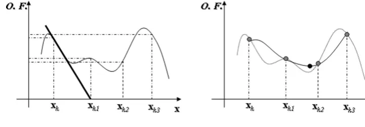
The gain sequence ak is computed using a Polynomial Interpolation (PI) of the objective function along the descen-dent direction: at each iteration the minimum point of the polynomial interpolation is considered as the sub-optimal solution of the problem, as shown in Fig.1.
3 Description of the experiments
Experiments have been conducted on the test-network report-ed in Fig.2, consisting of 8 links and 8 nodes, with three traffic signals (same cycle time and green time equally split between the incoming approaches) introduced to increase congestion.
In detail, the following information has been considered as input of the estimation process:
1. information on links: counts and measured speeds collect-ed at 5 count sections on the network (Fig.2);
2. information on routes: path travel times for different de-parture times of probe vehicles along one path connecting origin 2 to destination 4 (Fig.2);
3. information on demand: previous demand matrices (seed matrices) with different degrees of reliability and aggre-gate demand data (generated trips).
Counts, measured speeds and path travel times have been collected performing a dynamic user equilibrium assignment by DYNAMEQ [22], given a supposed“true”demand matrix, which is assumed to be unknown to the analyst. The total time horizon of the assignment is 50 min. The demand is charac-terized by three O-D components (between centroids 2 and 4, 6 and 4, 3 and 4, Fig.2) for a total amount of about 4,400 veh/
Fig. 2 Test network with count sections and paths of probe vehicles
Fig. 3 Demand profile for the“true”matrix and for some seed matrices
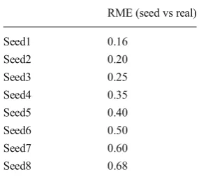
Table 1 Relative Mean Errors (RME) of the seed matrices used in the experiments
RME (seed vs real)
h and it has been divided into 5 time slices of 10 min each with a variable profile (Fig.3). Only one O-D component (from 2 to 4, Fig.2) has a possible route choice. Information on links (traffic counts and measured speeds) is collected every time slice, while path travel times have been collected only for the first three time slices.
Different seed matrices, representing possible a priori knowledge of demand have been obtained by random pertur-bations of the“true”matrix.
The distance between the“true”matrix and the seed matrix, which represents the reliability of the latter, has been comput-ed using the Relative Mean Error (RME) statistic:
RME ¼
X
i X
j
xri;j−di;j
xr i;j
where:
d “seed”demand values
xr “true”demand values
i time interval
j O-D pairs
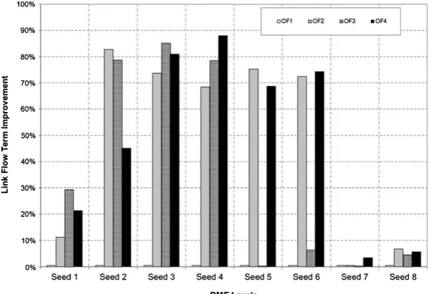
Fig. 4 Objective Function (OF) improvements for different degrees of reliability of the seed matrix
In particular, 8 seed matrices have been generated with a RME value ranging from 0.16 (high reliability) to 0.68 (low reliability), as reported in Table1.
In Fig.3the variable demand profiles of the“true”matrix and of some of the adopted seed matrices are reported: the differences between the profiles suggest the need to work not only on the value of the total demand, but also on its distri-bution between the time slices.
Four different objective functions (OF) have been defined, grouping the collected information in the following way:
– OF1: distance between simulated flows and link counts plus distance between estimated demand and seed matrix;
– OF2: distance between simulated flows and link counts, plus distance between simulated speeds and measured link speeds, plus distance between estimated demand and seed matrix;
– OF3: distance between simulated flows and link counts, plus distance between simulated path travel times and measured path travel times from probe vehicles, plus distance between estimated demand and seed matrix; – OF4: distance between simulated flows and link counts,
plus distance between simulated speeds and measured link speeds, plus distance between simulated path travel times and measured path travel times from probe vehicles, plus distance between estimated demand and seed matrix.
Fig. 6 Link speed term improvements for different degrees of reliability of the seed matrix
4 Results
Results of the SPSA AD-PI, for different degrees of reliability of the seed matrix and using different types of information inside the objective function, demonstrate the effectiveness of the procedure, with improvements of the objective function up to 50 %. Smaller improvements are experienced if the seed matrices have very low reliability (RME≥0.6, Seed 7 and Seed 8), because of the large distance from the real demand.
The following figures highlight the effects of different kinds of real-time information on the accuracy of O-D demand estimation, for different degrees of reliability of a priori infor-mation on O-D demand. The best improvements are obtained using OF4; that is, when path travel times are considered together with measures of speeds and flows on link sections. In particular, objective function improvements higher than 40 % are obtained for seed matrix reliability ranging from RME=0.2 to RME=0.5 (from Seed 2 to Seed 6 in Fig.4).
Only when RME is lower than 0.2 (Seed 1) OF4 does not present the best improvement: this due to the very high reli-ability of the seed matrix, which makes useless additional information to improve the solution.
Intermediate reliability levels (0.2≤RME≤0.4, Seed 2 to 4) show similar behaviour in terms of sensitivity to information. Analysing each term of the OFs, it can be underlined that OF2 and OF4 usually imply the highest improvement for the term relative to the distance between link flows and traffic counts (Fig.5).
It means that link speed measures and path travel time data are very useful to obtain a better correspondence with traffic counts. OF2 and OF4 show very similar improvements of the term relative to the link speed (Fig.6), a fact that demonstrates the capability of the two types of information (link speeds and path travel times) to represent the different levels of conges-tion of the network.
Finally, regarding path travel time term, OF3 and OF4 have similar improvements for low and medium degrees of reliabil-ity (RME≤0.4, Seeds 2–4, Fig.7). However, if RME is greater than 0.4, information on link speeds is no more sufficient to reflect the experienced path travel times.
It is possible to deduce from the previous considerations that for certain seed matrix reliability, the more information we add inside the adjustment procedure, the more accurate is the result. Of course, the accuracy of the estimation procedure can be only evaluated in laboratory experiments, where the true demand is known, while it is not possible in the real world, where only traffic measures are known.
So, the accuracy of the resulting demand is evaluated in the following pictures in terms of reduction of the distance be-tween estimated and real demand, for the different OFs adopted and for the different degrees of reliability of the seed matrix (Figs.8,9,10and11).
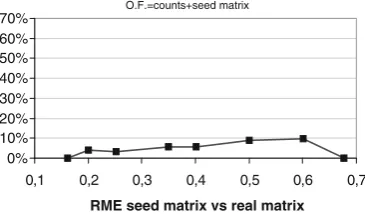
When real-time information includes only link fIows, as in case of OF1 (Fig.8), the improvement of the solution with respect to a priori information is lower than 10 %; if also measured link speeds are added inside the objective function as in case of OF2 (Fig.9), the improvement of initial estima-tion exceeds the 50 %, except for poor reliability of the boundary values of the seed matrix. This result highlights the importance of speed data on dynamic demand adjustment, as it allows to discriminate between congested or uncongested traffic conditions.
If data on path travel times instead of link speed are added to link counts (OF3, Fig.10) strong improvements are still obtained compared to using only link counts, even if lower than those obtained by using measured speeds (Fig. 9) and
O.F.=counts+seed matrix
0% 10% 20% 30% 40% 50% 60% 70%
0,1 0,2 0,3 0,4 0,5 0,6 0,7
RME seed matrix vs real matrix
Fig. 8 Improvement of the solution for different degrees of reliability of the seed matrix, in case of objective function taking into account the closeness to link counts and to the seed matrix (OF1)
O.F.=counts+measured speeds+seed matrix
0% 10% 20% 30% 40% 50% 60% 70%
0,1 0,2 0,3 0,4 0,5 0,6 0,7
RME seed matrix vs real matrix
Fig. 9 Improvement of the solution for different degrees of reliability of the seed matrix, in case of objective function taking into account the closeness to link counts, to measured link speeds and to the seed matrix (OF2)
O.F.=counts+measured travel times+seed matrix
0% 10% 20% 30% 40% 50% 60% 70%
0,1 0,2 0,3 0,4 0,5 0,6 0,7
RME seed matrix vs real matrix
concentrated in a small range of seed matrix reliability (RME from 0.2 to 0.35).
Finally, if both information on links (flows and speeds) and information on path travel times are put together (OF4, Fig. 11), an improvement is experienced increasing up to 66 % for RME equal to 0.35 and then decreasing to about 2 % when for RME equal to 0.68. So, speeds and path travel times add information to the adjustment process in order to reach a dynamic demand matrix closeness to the real one; however, their effects do not seem to be additive.
In order to better understand this result, it is necessary to explore the characteristics of the measures adopted inside the adjustment procedure in detail:
– regarding link measurements, we assume measures of flows and speeds on 5 count sections collected for 5 time intervals, for a total number of 50 data, which cover information related to all the origin–destination compo-nents of the network (Fig.2);
– regarding path travel times, we assume only one path covered by probe vehicles, which cover information on only one origin–destination pair, measured from the ori-gin for the first 3 time slices (that is, we assume that only a sample of vehicles are equipped with GPS devices and can be exploited as probes).
Measures are then normalized inside the objective func-tion; i.e., the information is not weighted for its cardinality; however, link measures provide information on all the origin– destination components, while path travel times only on one origin–destination pair.
Table2shows how the error of estimation for the origin– destination pair (2–4 in Fig.2) followed by the probe vehicles change for different levels of seed matrices reliability and for different objective functions. It is interesting to notice that the information on path travel times OF3 brings to the largest improvements in the estimation of the flow on the O-D pair 2– 4 when the seed matrix is related to RME values up to 0.35 (Table 2). For RME greater than 0.35, information on path travel times adds no improvement with respect to information on only link flows (OF1): this is also confirmed by Fig.10for the same range of RME. This last result can be explained considering that when a priori information has very low reliability, adding measurements on only one origin– destina-tion pair and three departure time intervals is not sufficient to achieve further information on the whole time-dependent O-D demand matrix. In fact, path travel times on the last departure times are lost and information on all the origin–destination pairs can be obtained only if speed measurements for the whole time period are added (OF4). Moreover, OF4 implies best proximity (except in Seed 2) between real and estimated demand values for the O-D pair 2–4 (Table2).
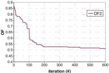
Finally, some remarks are reported about the convergence of the algorithm: SPSA AD-PI shows a good stability of the
Table 2 Difference between real and estimated O-D pair 2–4 [veh/h] for different degrees reliability of the seed matrix and different objective functions (O.F.)
RME (seed vs real) O.F.1 O.F.2 O.F.3 O.F.4
0.16 246 222 184 160 0.20 725 170 135 377 0.25 958 364 209 213 0.35 1,250 505 444 136 0.40 1,450 511 1,450 543 0.50 1,525 645 1,487 160 0.60 1,938 1,932 1,938 1,905 0.68 2,442 2,354 2,395 2,371
0.4 0.45 0.5 0.55 0.6 0.65 0.7 0.75 0.8 0.85 0.9
iteration (#)
OF
OF2
0 100 200 300 400 500 600
Fig. 12 Convergence of the objective function OF2
0.6 0.7 0.8 0.9 1 1.1 1.2 1.3 1.4
0 100 200 300 400 500 600
iteration (#)
OF
OF4
Fig. 13 Convergence of the objective function OF4
O.F.=counts+measured speeds+seed matrix+measured travel times
0% 10% 20% 30% 40% 50% 60% 70%
0,1 0,2 0,3 0,4 0,5 0,6 0,7
RME seed matrix vs real matrix
objective function after 200÷300 iterations, as reported in Figs.12and13, relative to OF2 and OF4, respectively.
Each iteration takes about 1 min on a Dual Core, 2.2 GHz machine; this means about 4 h are needed to solve the opti-mization problem for the test network reported in this study. If the dimension of the network increases, also computational times increase because of the time needed by the DTA simu-lator to generate simulated values of measures at each itera-tion. As a result, the procedure can be used only in off-line context. However, the solution found can be exploited as first input for on-line applications in order to start with good initial demand values and good traffic flow patterns on the network.
5 Conclusion
The paper has presented a preliminary analysis on the contri-bution provided by different kinds of information to the esti-mation of time-dependent O-D matrix demand. Numerical experiments carried out on a test-network case demonstrated the importance of type, quality and quantity of the information in demand estimation.
The best improvements on demand adjustment are usually obtained when a sample of path travel time measurements is considered together with measures of speeds and flows on link sections. In fact, link speeds and path travel times allow taking into account traffic congestion, which affects the propagation of flow on the network and then influences the time-dependent relationship between link counts and O-D demand matrix. Numerical experiments highlighted also the influence of the reliability of a priori information on the accuracy of resulting O-D estimation in combination with different information sets. Further research will be addressed to investigate the influ-ence of penetration rate of probe vehicles that provide infor-mation on path travel times, considering also higher dimen-sion networks; moreover the effect of other kinds of measure-ments, like density and occupancy, as well as point-to-point travel time data, which introduce additional information on network congestion, will be analysed
Open Access This article is distributed under the terms of the Creative Commons Attribution License which permits any use, distribution, and reproduction in any medium, provided the original author(s) and the source are credited.
References
1. Di Gangi M, Croce A (2005). Combining simulative and statistical approach for short time flow forecasting. Association for European Transport and contributors
2. Etemadnia H, Abdelghany K (2009) Distributed approach for esti-mation of dynamic origin–destination demand. Transp Res Record: J Transp Res Board 2105:127–134
3. Zhou X, Mahmassani HS (2004). Recursive approaches for online consistency checking and o-d demand updating for realtime dynamic traffic assignment operation. 84th Annual Meeting of the Transpor-tation Research Board
4. Barceló J, Montero L, Marqués L, Carmona C (2010). A kalman-filter approach for dynamic od estimation in corridors based on bluetooth and wifi data collection, 12th WCTR
5. Bierlaire M, Crittin F (2004) An efficient algorithm for real-time estimation and prediction of dynamic OD tables. Oper Res 52(1):116–127
6. Cipriani E, Fusco G, Gori S, Petrelli M (2006). Heuristic methods for the optimal location of road traffic monitoring stations. Proc. of IEEE Intelligent Transportation Systems Conference, 2006. ITSC’06, pp. 1072–1077
7. Balakrishna R (2006). Off-line calibration of dynamic traffic assign-ment models. PHD thesis. Massachusetts Institute of Technology 8. Cipriani E, Florian M, Mahut M, Nigro M (2010). Investigating the
efficiency of a gradient approximation approach for solution of dynamic demand estimation problem. New Developments In Trans-port Planning—Advances in Dynamic Traffic Assignment, edited by Tampère, Viti and Immers
9. Cipriani E, Florian M, Mahut M, Nigro M (2011) A gradient approx-imation approach for adjusting temporal origin–destination matrices. Transp Res Part C 19(2011):270–282
10. Dixon M, Rilett LR (2002) Real-time OD estimation using automatic vehicle identification and traffic count data. Comput-Aided Civil Infrastruct Eng 17(2002):7–21
11. Eisenman SM, List GF (2004) Using probe data to estimate OD Matrices. Intelligent transportation systems conference. Washington DC 3–6:291–296
12. Antoniou C, Ben-Akiva M, Koutsopoulos HN (2004) Incorporating automated vehicle identification data into origin–destination estima-tion. Trans Res Rec: J Transp Res Board 1882:37–44
13. Zhou X, Mahmassani HS (2006) Dynamic origin–destination de-mand estimation using automatic vehicle identification data. IEEE Trans Intell Transp Syst 7(1):105–114
14. Caceres N, Wideberg JP, Benitez FG (2007) Deriving origin– desti-nation data from a mobile phone network. IET Intell Transp Syst 1(1):15–26
15. Barceló J, Montero L, Bullejos M, Serch O, Carmona C (2012). Dynamic OD matrix estimation exploiting bluetooth data in urban networks, Recent researches in automatic control and electronics, ISBN: 978-1-61804-080-0
16. Mitsakis E, Salanova JM, Chrysohoou E, Aifadopoulou G (2013). A robust method for real-time estimation of travel times for dense urban road networks using point-to-point detectors. Proceedings of the 92nd Annual Meeting in Transportation Research Board, TRB 2013
17. Iannò D, Postorino MN (2002). A generation constrained approach for the estimation of O/D trip matrices from traffic counts
18. Zhou X, Lu C, Zhang K (2012). Dynamic origin–destination demand flow estimation utilizing heterogeneous data sources under Congested Traffic Conditions, Available online at: http:// onlinepubs.trb.org/onlinepubs/conferences/2012/4thITM/Papers-A/ 0117-000097.pdf. Accessed January 2013
19. Toledo T, Kolechkina T (2012) Estimation of dynamic origin– desti-nation matrices using linear assignment matrix approximations. IEEE Trans Intell Transp Syst Digit Object Identifier. doi:10.1109/TITS. 2012.2226211
21. Cascetta E, Inaudi D, Marquis G (1993) Dynamic estimators of origin–destination matrices using traffic counts. Transp Sci 27(4):363–373
22. Florian M, Mahut M, Tremblay N (2006). A simulation-based dy-namic traffic assignment model: Dynameq. In: Proceedings of the
First International Symposium on Dynamic Traffic Assignment DTA2006. Institute for Transport Studies, University of Leeds 23. Frederix R, Viti F, Corthout R, Tampère CMJ (2011) New gradient