ORIGINAL PAPER
Prioritization in modal shift: determining a region
’
s most suitable
freight flows
Dries Meers1&Cathy Macharis1
Received: 19 December 2014 / Accepted: 3 June 2015 / Published online: 26 June 2015
#The Author(s) 2015. This article is published with open access at SpringerLink.com
Abstract
PurposeDifferent policy measures have been introduced to enhance a modal shift from road-only to intermodal transport. In Northwestern European countries such as Belgium, policy makers are increasingly trying to approach shippers on an individual basis in order to convince them about the potential benefits of intermodal transport for their company. This paper proposes a tool to identify the most promising cases for modal shift in a predetermined region.
MethodsThe suggested methodology takes the form of a Geographic Information System-based macro-scan. It ranks geographic entities (or companies within) according to their modal shift potential, based on a list of space- and network-dependent criteria, such as transport volumes, transport price, post haulage transport time and product characteristics.
Results The methodology was applied to a transboundary case study in Belgium and the Netherlands. The results of the analysis can serve as input for a micro-scan that identifies the suitable companies in the most favorable areas. A sensi-tivity analysis is performed to check the robustness of the weights given to the considered criteria.
Conclusions The proposed methodology allows ranking geo-graphic entities according to their modal shift potential, pro-viding a strong tool to policy makers to focus their modal shift efforts on a limited number of transport flows with a high success rate. The practical usefulness of the results of the
analysis is however highly dependent on the quality and the level of detail of the transport flows input data.
Keywords Intermodal transport . Modal shift . Location analysis . Prioritization . Transport flows analysis
1 Introduction
Inter-port competition increasingly focuses on the hinterland legs of door-to-door transport chains through the integration of maritime and inland transport systems [1,2]. Vermeiren [3], studying competition between the ports of Rotterdam and Antwerp, even claims that intermodal transport chains are the single key differentiators in these door-to-door transport chains. Nevertheless, most ports (have to) rely to a large extent on road transport for serving their hinterland, although inter-modal transport connections can maintain and extend the hin-terland of seaports [4]. In this research, intermodal transport is defined as the use of different transport modes in a single transport chain, using loading units such as standardized con-tainers, with no handling of the goods when changing modes (based on [5]) and the focus is solely on hinterland chains. An extensive intermodal transport network gives logistics service providers the opportunity to offer shippers a wide range of transport possibilities [6]. Furthermore, these alternative trans-port modes can alleviate congestion problems in and around the port area. Different barriers however prevent a more ex-tensive use of intermodal transport services (see e.g. [7–9]).
Additionally, the European Commission is aiming to shift road freight transport to more sustainable transport modes [10, 11]. Policy makers on national and regional levels and port authorities have made significant efforts to shift goods from road to rail, inland navigation and short sea shipping. In many cases, these modal shift policies aim at a wide audience of
* Dries Meers
Cathy Macharis
1 MOBI - Mobility, Logistics and Automotive Technology Research
potential beneficiaries, using policy instruments such as taxa-tion, regulataxa-tion, infrastructural measures or the granting of financial incentives [12]. In countries such as Belgium and the Netherlands, policy makers also demand transport consul-tants to approach individual companies and assist them in the start-up of using intermodal transport services [13,14]. Un-fortunately, however, the current modal share of these alterna-tive modes remains modest in most European regions. In the Flanders region in Belgium for instance, the 2011 modal share of road freight transport, expressed in ton-km, was still esti-mated to be around 81 % compared to 9 % for rail and 10 % for inland waterways [15].
Following the rationale of individually guiding companies in exploring modal shift opportunities, this paper tackles the research problem of identifying a region’s most promising freight flows for modal shift to intermodal transport services. To tackle this problem, a methodology is proposed that ranks the transport flows yielding the greatest potential for modal shift in a studied region, based on a set of quantitative criteria. In complement with other modal shift analyses (e.g. [16]), the aim is not to identify the total potential for modal shift in a region or solely to identify whether intermodal transport can be cost competitive, but instead to compare different transport flows and rank them based on their affinity for a modal shift. The main rationale to do so is that the most highly ranked companies—or the companies located in the most highly ranked places—can be approached and guided in their modal shift efforts by transport consultants. The goal is to identify the shippers which are most likely to benefit from a modal shift. These shippers are more likely to be willing to switch to in-termodal transport services. But often they are unaware of its potential or they are hindered by red tape.
The following section of this paper describes different tools that can be used to estimate the potential for modal shift in a region and identifies the parameters affecting transport mode choice decisions. The third section describes in more detail the methodology elaborated in this paper, consisting of two main parts: a transport flows analysis and a spatial evaluation. In the fourth section, the methodology is applied to a case study, concentrating on two provinces both named Limburg, one in the east of Belgium and the other one adjacent, in the south of the Netherlands. The focus is on container transport to and from the Port of Antwerp.1The motorways connecting the provinces to this port suffer from severe congestion [17] de-spite the fact that intermodal barge transport is available as an alternative. A final section concludes the article and provides recommendations for future research.
2 Estimating the modal shift potential
Intermodal freight transport, employing alternative transport modes such as rail and inland waterway transport for the main part of the transport chain, with the pre- and/or post haulage of the trip performed by truck, has been promoted by policy makers and academics, as intermodal transport is in most cases considered to have a smaller impact on society [18]. Shifting freight from road transport to these alternative trans-port modes has therefore been a policy objective of the Euro-pean Commission in the past decades (e.g. [11,19]). Public authorities possess a range of policy instruments to increase the use of intermodal freight transport. As infrastructure pro-viders, authorities can try to accommodate an extensive and accessible infrastructure network, which brings the opportuni-ty to use intermodal transport chains to more potential users. Next, legislations can aid in efforts regarding interoperability, standardization and harmonization to facilitate fluent transport chains. Price incentives through (start-up) subsidies [20,21] or a (partial) internalization of external transport costs [18,22] can increase the price incentives to use intermodal transport. Investments in technology and innovations can contribute to an increased modal share on a longer term. Promotion of the intermodal sector can also be done on a more individual basis. Promotion offices assist in providing accurate and up-to-date information to potential customers, enhance a mind shift and convince potential users by demonstrating good practices [23, 24]. Benchmarking tools, such as the one developed in the BE LOGIC project [25,26] that uses six key performance indica-tors to compare unimodal to intermodal transport services, are available to analyze freight flows on a company level. This tool gives users the opportunity to assign weights to perfor-mance indicators to determine case-specific modal choice preferences.
In Northwestern European countries such as Belgium and the Netherlands, modal shift policies have partly shifted to-wards an individual guidance of companies in order to in-crease the awareness on the possibilities of using intermodal transport chains. Already in 2000 a logistics scan was per-formed to assess a modal shift for 100 shippers in the Nether-lands [13]. From 2006, transport experts commissioned by the Flanders’Chamber of Commerce and Industry started helping individual companies in the assessment of transport options, using inland waterway transport and short sea shipping. In 2013, a project was set up by the Flanders region to employ logistics consultants, whose goal is to assist companies in reducing costs and increasing efficiency, by inter alia using intermodal transport solutions [14]. To aid these consultants in their daily work, different tools can be used in a preparatory phase to scan the modal shift potential of a region and identify the transport flows most suitable for modal shift. This section provides an overview of, and the rationale for, such macro-tools and of the criteria that should be included in these macro-tools. 1A similar analysis was performed for container transport to
Eng-Larsson and Kohn [27] find that three factors influ-ence the decision to change transport modes: business strate-gies, the logistics systems design and external pressures such as environmental legislation. Further, an extensive amount of literature exists on modal choice criteria, estimating the influ-ence of different parameters such as transport cost and trans-port time (for an overview see [28]).
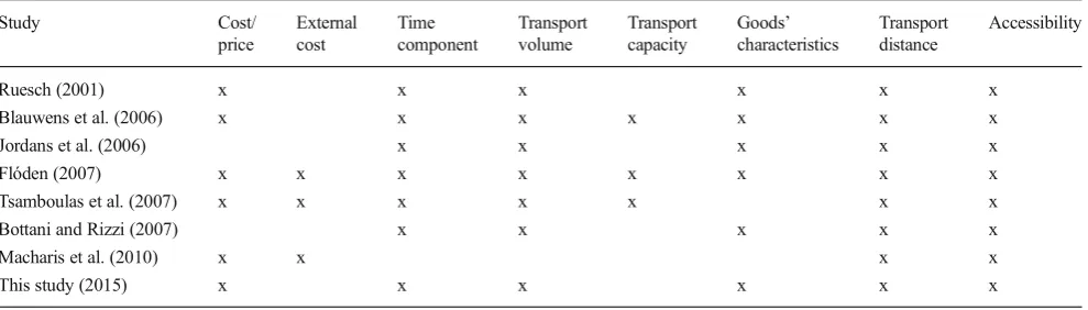
Different models have been developed to estimate the im-pact of modal shift policies on the use of intermodal transport combinations. Several review papers discuss the operation research models [29–31] and decision support systems [32, 33] used for the analysis of intermodal transport systems. Macharis et al. [18] investigate the influence of increased fuel prices and an internalization of external transport costs on the market areas of intermodal transshipment terminals in Bel-gium, using an all-or-nothing flow assignment based on a shortest path algorithm and price minimization. Their model allows for calculating the environmental gains and cost sav-ings of a modal shift in a certain area. Blauwens et al. [34] present a similar approach as they assess the effectiveness of different policies based on total logistics costs, incorporating time components in the cost function. Both studies conclude that a combination of policy measures can lead to significant modal shifts from road to intermodal transport. Additionally, the Heuristics Intermodal Transport model, developed by Flodén [35], allows one to analyze the effect of several policy measures on modal shares and can indicate regions with strong potential for intermodal transport. den Boer et al. [36] estimate the potential for a modal shift from road to rail trans-port in Europe and the corresponding total greenhouse gas emission savings, based on existing studies, extrapolations of relevant case studies and an infrastructure capacity analysis. An overview of the parameters included in these studies is given in Table1.
Tsamboulas et al. [22] propose a three step methodology to asses the possible impact of a policy measure to induce a modal shift on a European scale. A first step consists of a macro-scan which assesses the potential for modal shift. This toolbox compares cost- and quality-related mode choice
criteria. The methodology also includes sensitivity analyses and finally results in a policy action plan. A methodology to calculate the‘basic potential’for each transport mode is pre-sented by Jordans et al. [37] for the case of the Netherlands. They apply a fivefold filter to find the goods flows that qualify for a modal shift. These filters are: accessibility to a transship-ment terminal, transport-mode dependent break-even dis-tances, product type characteristics, shipment size and trans-port speed requirements. They estimated the potential of rail-, barge- and short sea transport to be 33.5 % of the total tonnage transported.
Ruesch [38] presents a methodology to identify the poten-tial for modal shift, considering both the demand and the sup-ply side. A macro approach analyses aggregated freight flows on different geographic levels. Product characteristics are accounted for by using aptitude factors related to the commod-ity types transported. Cost comparisons are made using gen-eralized cost functions, accounting for transport cost and time. The next step consists of a micro approach, which identifies the true potential based on a freight flow and logistics chains analysis on company level. Finally, Bottani and Rizzi [16] propose a methodology to calculate the potential volume that a new intermodal terminal could attract. This potential is cal-culated as the share of the current road transport that can divert to intermodal rail transport. For each transport flow, an affinity score is calculated which assesses the likelihood of a modal shift. To calculate this score, three characteristics of the pos-sible transport chains are included: the break-even transport distance, the time of the potential post-haul transport and the aptitude of the type of goods transported. Service characteris-tics are not explicitly included, as they are assumed to be equal for the available alternatives.
The methodology proposed in this paper builds on these previous studies. It follows the approach of the macro-scan presented by Ruesch [38] which serves as the input for a micro-scan on company level. To determine the modal shift potential, the assessment criteria were derived from the work of Bottani and Rizzi [16]. A main difference in this paper is however that the methodology is altered to rank freight flows
Table 1 Overview of modal shift determinants (explicitly) included in relevant studies
Study Cost/
price
External cost
Time component
Transport volume
Transport capacity
Goods’ characteristics
Transport distance
Accessibility
Ruesch (2001) x x x x x x
Blauwens et al. (2006) x x x x x x x
Jordans et al. (2006) x x x x x
Flóden (2007) x x x x x x x x
Tsamboulas et al. (2007) x x x x x x x
Bottani and Rizzi (2007) x x x x x
Macharis et al. (2010) x x x x
according to their potential for modal shift from greater to smaller. By using the Location Analysis Model for Belgian Intermodal Terminals (LAMBIT), developed by Macharis [39], transport prices can be included in the analysis to check whether intermodal transport can be price competitive for transport to a given geographic entity. The criteria which are included besides price are: the post haulage transport time, product characteristics and the extent of the current flows transported by road (volume and commodity types transported). Accessibility and transport distance are implicit-ly included as they (partimplicit-ly) determine transport price and time. Transport capacity is not explicitly included in the analysis, as no information on free vehicle capacity is available and be-cause frequency of intermodal services can be augmented to increase transport capacity in the presented case study. This criterion could, however, be included when terminal capacity is a limiting factor. How the previous criteria are calculated and used to rank transport flows on their modal shift potential is elaborated in the following section.
3 Methodology
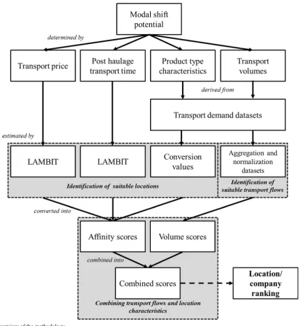
The macro-scan approach elaborated in this paper comprises two main parts that are combined to rank transport flows ac-cording to their modal shift potential. The first part consists of the identification of the biggest transport volumes, by com-bining information from different datasets containing origin– destination information. In a second step, a location-specific affinity score for a modal shift to inland waterways transport is calculated based on estimated transport prices and post haul-age transport times. When combined with the transport vol-ume information, it allows for the comparison and ranking of companies located in different places on their qualification for modal shift. A general overview of the methodology is pre-sented in Fig.1. Each downward arrow indicates a calculation and or an assumption, which is explained and motivated in more detail in the followings sections. The first assumption is thus that the modal shift potential can be determined based on the criteria of price, transport time, product characteristics and transport volume. This assumption follows the work of Bottani and Rizzi [16], with the main difference being that they use transport distance as a proxy for transport price/cost.
3.1 Identification of suitable transport flows
To identify the transport flows with the greatest potential for modal shift, transport demand datasets are analyzed (see Fig. 1). Different data sources provide information on the origin, destination and loading unit of transport flows. Map-ping these datasets can show the spatial spread of relevant volumes and will serve as input for the macro-scan of the region. As indicated above, the volume of the flows and the
product characteristics strongly influence the modal shift po-tential, as intermodal transport is based on the principle of economies of scale to reduce the transport cost per transported loading unit. Sometimes low density high value goods can also be transported by intermodal solutions when logistics and quality requirements can be met [40].
To determine the potential for modal shift, the focus in this research is solely on goods currently transported in containers from the sea port to the hinterland by trucks. In theory, other transports can also qualify for modal shift. These transport flows are however not explicitly considered in this analysis, as goods that are already transported in containers from door-to-door have a higher chance to shift from road to inland waterways or rail, and the focus is on quick wins.
As large-scale and detailed datasets on freight flows are often scarce, background information on the available data sources should be gathered and only appropriate data sources are to be selected for the analysis. For the case study described in the next section, the data sources were selected based on information availability concerning: (i) the origin and destina-tion of relevant transport flows; (ii) the type of loading unit (e.g. containers); (iii) the year of reference (maximum 5 years ago); (iv) the geographic level of detail of origin and destina-tion (e.g. NUTS3); (v) the unit expressing the transport vol-umes and (vi) the product type. Few datasets, however, in-clude information on this latter criterion. Therefore, relevant datasets not including product information are not excluded. The accuracy and the reliability of the results of this analysis will thus depend on the extent to which these available datasets represent real-life transport flows.
In the case study described below, three datasets are includ-ed; each having specific advantages and disadvantages (see Table3). Combining these datasets allows for a more nuanced image of the existing transport flows in the study area. How-ever, data manipulation is needed to put the datasets to a clear comparison base. This manipulation consists of four steps, described below (see Fig.2for a fictitious example).
The different datasets are expressed in different units (tons or TEU) and different extrapolation methods have been used to convert the sample into the final dataset. Therefore, in the first step, it is calculated for each dataset separately which share of the total transport flows leaves and arrives in each geographic entity. This is done to overcome over- or underes-timations of the total volume transported, mentioned in each dataset.
Other parameters such as the number of companies or the added value produced could possibly be used for this normal-ization if a clear link to the transported volume can be proven. The third step consists of an aggregation/disaggregation of the datasets. As the origins and destinations of the datasets are not always expressed at the same geographical level they are hard to compare. In the case study described below, all infor-mation was converted to the municipal level. This meant that, for instance, the Eurostat data were disaggregated, assuming an equal distribution of the flows over the original entity. If available, it would however be useful to employ an indicator of the spatial spread of these flows for a more accurate distribution.
of volume density. For the fictitious example in Fig.2, one can conclude that the entityA1has a greater modal shift potential
thanA2. In regionB, both entities have an equal V-Score.
3.2 Identification of suitable locations
Besides the characteristics of the transport flows (volume and type of goods transported), the potential for modal shift can also be determined by locational characteristics of the origin and destination. In the modal choice literature, a distinction is made between cost- and quality-related variables [42]. The co st for intermodal t ransport mainly de pe nd s o n
infrastructure-related characteristics (transport distance, loca-tion of transshipment facilities, accessibility etc.) and the vol-ume transported. Some of the quality-related criteria also de-pend on the infrastructure availability, such as transport time, while others are related to the volume transported, such as service frequency. Other criteria cannot easily be linked to the infrastructure or transport volume. It is assumed in this analysis that these intermodal transport characteristics are rat-ed equally good for all intermodal alternatives. The geograph-ic entities with the greatest potential for modal shift can there-fore be derived from comparing infrastructure-related param-eters, product characteristics and transport volumes.
As described above, the criteria used in this analysis are based on the ones proposed by Bottani and Rizzi [16]. They use the parameters of transport distance, post-haul transport time and the characteristics of the products that are transported to/from these locations to give an estimation of the competiveness of intermodal rail transport compared to road-only transport, as they assume that intermodal transport is only profitable over longer distances, while short post-haul transport times decrease the total logistics cost. Instead of transport distances, in this analysis transport price ratios are compared to provide insight into the price competitiveness of intermodal barge transport in different locations. Values for each of these three parameters are calculated for each geo-graphic entity in the studied region. To combine this informa-tion with the volume scores derived in the previous step, the same geographic level of detail is required.
To include transport prices, a price index comparing the cheapest intermodal route to the cheapest unimodal road trans-port route is created. The lower this index the higher the af-finity for a modal shift will be. These prices are calculated using the LAMBIT model, developed by Macharis [39]. LAMBIT is a Geographic Information Systems-based model that calculates the cheapest transport alternatives based on a cheapest path algorithm, which is comparable to the shortest path algorithm developed by Dijkstra [43]. The model thus uses the existing networks of the different transport modes to calculate cheapest transport routes for all modal alternatives. These include the origin and destination locations, the road and inland waterways networks and the inland terminals which allow switching between modes. Rail transport net-works can also be included but were not relevant for the case study described below. In the case study, the center points of the municipalities in the research area, as proxy for the com-plete entity, and the geographic center of the Port of Antwerp are considered as origins or destinations of the transport flows. The routes between origin and destinations are calculated based on distance-depended price functions which are derived from surveys. The function used for the intermodal transport simulations consists of a fixed component (e.g. transshipment prices) and two variable components, which are dependent on the distance of the main haul transport by barge and of the Fig. 2 Overview of the methodology, applied to a fictitious example. In
distance of the post-haul transport by truck. For transport be-tween a port and its hinterland, the model will calculate the cheapest transport alternative by road transport and by inter-modal barge transport. By comparing these prices per geo-graphic entity (e.g. municipalities), the price index is calculat-ed. LAMBIT has been used and tested previously to calculate the impact of policy measures on transport prices and on the market area of intermodal terminals (e.g. [18,20]) and to determine the optimal location for new intermodal terminals [44]. The calculation of the price ratio on municipal level is described in Pekin et al. [45]. For the case study described below, the model was geographically extended to include the neighboring countries of Belgium.
The LAMBIT model is also used to calculate the estimated transport time of the post-haul transport. This post-haul trans-port time also gives an indication of the reliability of an on-time delivery. To calculate this value, detailed information on congestion should however be available for analysis. As this was not the case for the case study below, it was assumed that the post haul transport is always performed at an average speed of 60 km/h. The post-haul transport distance was de-rived from the routes simulated with LAMBIT to determine the transport price of the cheapest intermodal alternative and used to calculate the average post-haul transport time for each geographic entity.
Finally, information on the product characteristics is in-cluded when available. Bottani and Rizzi [16] calculated the aptitude of goods categories to be transshipped in an inter-modal terminal. They asked terminal managers to make judg-ments using a Likert scale which they transformed into a sin-gle coefficient per goods category. These coefficients are matched with the goods classifications of the available datasets in this analysis. Dependent on the volume of transport flows to/from a given location, an average aptitude coefficient is calculated for the total of transport flows to/from each geo-graphic entity.
3.3 Combining transport flows and location characteristics
Finally, the results of the volume analysis and the location analysis are combined (see Fig.1). Bottani and Rizzi [16] combine different input parameters to calculate an‘affinity
index’of given transport flows. In this case, the affinity for a modal shift of a geographic entity is calculated, based on similar, but altered input parameters.
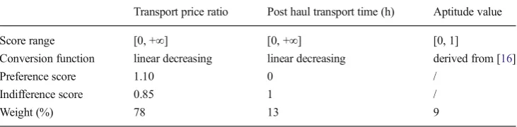
The V-score is multiplied by an affinity score, ranging from 0 to 1, which is derived from the location analysis. As the price ratio, post-haul transport time and aptitude values cannot directly be summed; each time and price score is converted into a score within a 0 to 1 range. A value of 1 indicates a maximum affinity for modal shift, while the 0 value corre-sponds to no affinity for modal shift. The conversion of these three scores into a single affinity score can be interpreted as a multi-criteria evaluation, as presented by Meers et al. [46]. In this case, linear decreasing functions were assumed for the conversions of the transport price ratio and the post-haul trans-port time (see Table2). An intermodal/unimodal price ratio of 0.85 or higher for instance matches a score of 1 and price ratios equal or above 1.10 match a score of 0. All negative scores were also set at 0. For the time parameter, 1 h of post-haulage, or more, matches a score of 0, while a post-haulage time of 0 min matches a score of 1. The aptitude scores, de-rived from Bottani and Rizzi [16] were already converted within this 0–1 interval and so did not need any conversion. It should however be noted that the conversion rates of the different variables can influence the results of the analysis. An analytical validation of these assumptions would be useful, but in this research the proposed values were validated by the steering committee of the project. Next, the price -, time –and aptitude scores were combined into a final affinity score, based on the weights derived from Bottani and Rizzi [16], given to each parameter influencing the total affinity: distance/price (78 %), time (13 %) and product aptitude (9 %). The combined score for each location, which allows ranking all entities on their modal shift potential, was then obtained by multiplying the location-specific V-score by the location-specific total affinity score (see Fig.1).
4 Limburg case study
The proposed methodology was applied to a case study for transport between the Port of Antwerp and the provinces of Limburg in Belgium and the Netherlands. The current share of barge transport in the modal split of hinterland transport of the
Table 2 Determinants for the multi-criteria conversion of criteria scores to a general affinity-score
Transport price ratio Post haul transport time (h) Aptitude value
Score range [0, +∞] [0, +∞] [0, 1]
Conversion function linear decreasing linear decreasing derived from [16]
Preference score 1.10 0 /
Indifference score 0.85 1 /
Port of Antwerp is 36 %, compared to 57 % for road and 7 % for rail [47]. Originally transport flows between these regions and the Port of Rotterdam were also analyzed, but due to the lower data quality, they were not included in this case study.
The study area included both provinces of Limburg, but to frame the modal shift potential in a broader context, the area within a 50 km radius of these provinces was also included in the study area. The policy objective of the study was to find promising modal shift cases within the two provinces using local transshipment terminals. For this reason, not all trans-shipment terminals in the study area were included in the analysis. Only the terminals in Limburg with regular barge connections to the Port of Antwerp were considered, these being: Venlo, Venray, Stein and Born in the Netherlands and Genk and Beringen in Belgium. In addition, the terminal in Meerhout was also included, following its location just across the province border. As these terminals are currently not op-erating at full capacity, or extensions are planned, no trans-shipment capacity limits were accounted for. These terminals are connected to the port through the Albert Canal in Belgium, the Meuse and the Juliana Canal in the Netherlands and some smaller canals. Possible competition with intermodal rail transport was not included in the analysis, due to the focus on short distance transport.
To identify the most suitable transport flows, three datasets were considered (Table3). A first dataset was retrieved from the Directorate General Statistics and Economic Information (DGSEI). This dataset provides very detailed information on freight transport within Belgium, but transport operations per-formed by trucks registered in other countries are not included in this dataset, decreasing the accurateness of the dataset in particular for international transport. Also, cabotage is not accounted for. The Eurostat dataset, on the other hand, yields data from all countries in the European Union and therefore overcomes this problem. The geographic level of detail on the origin and destination locations is however much lower. The third dataset is derived from the Port of Antwerp and contains very detailed information on the origin and destination of the container flows. Due to the limited duration of the data sam-pling, certain transport flows can be over- or
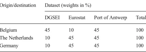
under-represented in this dataset. The weights attached to the differ-ent datasets are clearly linked to the estimated accurateness of the datasets (Table4).
The combined transport datasets resulted in the V-Scores for transport to/from the Port of Antwerp (Fig.3). It is clear that a high amount of containers is transported by road on rather short distances. Within Belgian Limburg, the highest road transport volumes go to and from a central axis, north of the Albert Canal and to some municipalities in the north and the south of the province. The highest concentrations in Dutch Limburg are found in the south, along the border with Belgian Limburg. Some municipalities, such as Venlo are local hotspots.
The affinity score was calculated as described above. But due to the fact that only one dataset contains product type information, the aptitude for modal shift could only be derived from the DGSEI dataset (Table3). The average aptitude for transport to the Belgian municipalities in the research area was 0.578. This average value was also used for municipalities that according to the DGSEI dataset did not receive any goods, but were included in other datasets.
Due to the large weight attached to price in the affinity score (78 % in Fig. 4), the municipalities with the highest scores are mainly in accordance to the market areas of the intermodal terminals (see also [45]). The municipalities with the highest affinity scores can indeed be found in the vicinity of the terminals of Genk, Stein and Beringen. Further, it should be noted that only the terminals mentioned in the figure are included as possible transshipment terminals in the Table 3 Container flow datasets
Dataset Reference year
Level of detail in Belgium
Level of detail abroad
Sampling method Type of goods characteristics
Unit
DGSEI 2011 LAU 2 NUTS 3 Weekly at random sample of 1000 Belgian trucks
Yes Tons
EUROSTAT 2011 NUTS 3 NUTS 3 Derived from individual countries No Tons Container
counts
2010 Zip code Zip code 3 day counts of trucks entering/leaving port terminals
No TEU
Table 4 Weights assigned to the different datasets
Origin/destination Dataset (weights in %)
DGSEI Eurostat Port of Antwerp Total
Belgium 45 10 45 100
The Netherlands 10 45 45 100
analysis, which explains the low affinity scores in remote mu-nicipalities. Adding the other transshipment terminals in and close to the case study region would indeed increase the affin-ity scores of these municipalities.
Finally the two map images can be combined into a single image (Fig. 5). The V-Score of each municipality is weighted based on its total affinity score, ranging from
0 to 1. For the given set of parameters, the highest scores in Limburg are found in municipalities in the center of Belgian Limburg, and in Dutch Limburg in the south of the province, bordering Belgium. Also, the municipality of Venlo scores high. The results can be ranked compar-ing the modal shift potential of all analyzed municipali-ties. In addition, a sensitivity analysis could be performed Fig. 3 V-Scores for transport to
and from the Port of Antwerp (Figs.3,4and5only display the intermodal terminals that were included in the analysis. They also only depict the inland waterways that are most relevant for the analysis.). In the Belgian part of Limburg, scores are highest in the center, while the scores in Dutch Limburg are higher in the east of Belgian Limburg and in the northeast of the province (based on [41])
to check the robustness of the results. This analysis can check for the effect of changing the price, time and apti-tude parameters, but the weight given to each parameter can also be varied as shown in Fig.6. The ten municipal-ities scoring best on the original ranking each time rank within the 20 best municipalities out of 440, under differ-ent weight distributions. When higher weights are given to the aptitude and time, five additional municipalities reach the top ten of best ranked municipalities. The graph shows that the results of the ten best ranked municipalities are robust, when weights are altered.
In a follow-up study, the municipalities with the highest rankings are scanned to list the companies eligible for a modal shift.2These companies are contacted and questioned on their possible interest in a modal shift. The shippers controlling the most promising transport flows could then be individually guided in a modal shift. When questioning these companies it can nevertheless become clear that due to company-related characteristics intermodal transport becomes less attractive, despite their high affinity scores.
5 Conclusions
In this paper, a methodology is presented that identifies the transport flows with the highest potential for a modal shift from unimodal road transport to intermodal barge transport. The aim is in a first stage to rank geographic entities, such as municipalities in the presented case study, according to the modal shift potential of the transport flows leaving and arriv-ing in the entity. This enables one to approach the companies generating flows with the highest estimated modal shift suc-cess rates in a second stage. This new methodology is also very interesting to guide companies in search for a suitable business location with a good intermodal accessibility.
To identify the most suitable locations or companies, dif-ferent parameters are included in the analysis: container vol-umes currently transported by road transport, the prices of Fig. 6 Ranking of the ten highest ranked municipalities under different
weight scenarios. Thedotted line(s)represent Dutch municipalities. Each scenario is represented as:Ranking weight LAMBIT score–weight time score–weight aptitude score
Fig. 5 Combined scores for transport to and from the Port of Antwerp
2The results of this micro-scan are not included in this paper but can be found
unimodal road transport and their intermodal alternative, the time required for the post-haul transport and the type of goods transported. The transport volume parameter was estimated by combining different datasets, resulting in a V-Score on munic-ipality level. The price comparison parameter and the time for post haulage were estimated, using the intermodal location analysis model LAMBIT.
The case study showed the importance of short post haul-age distances for the competitiveness of intermodal transport. A dense network of terminals located at strategic locations is thus an important asset for a region and for the possibility for organizing more sustainable transport via barge and to attract new companies. A sensitivity analysis showed the robustness of the results of the case study. The reliability of the results depends on the accurateness of the analyzed datasets and on the estimation of the parameters and their weights which rely to a great extent on expert judgment. This should be consid-ered when the methodology would be applied to other case study regions of which less accurate data is available.
Acknowledgments We gratefully acknowledge Provinciale Ontwikkelingsmaatschappij (POM) Limburg and Kamer van Koophandel for supporting this research project under the INTERREG IV framework‘Grenzeloze Logistiek’in the‘Impact project’, Phidan SA for the research collaboration, and DGSEI and the Port of Antwerp for providing the necessary input data.
Open AccessThis article is distributed under the terms of the Creative Commons Attribution License which permits any use, distribution and reproduction in any medium, provided the original author(s) and source are credited.
References
1. Notteboom TE, Rodrigue J (2005) Port regionalization: towards a new phase in port development. Marit Policy Manag. doi:10.1080/ 03088830500139885
2. McCalla RJ (1999) Global change, local pain: intermodal seaport terminals and their service areas. J Transp Geogr. doi:10.1016/ S0966-6923(99)00017-4
3. Vermeiren T (2013) Intermodal transport - The delta in the Delta. Dissertation, Vrije Universiteit Brussel
4. van Klink HA, van den Berg GC (1998) Gateways and intermodalism. J Transp Geogr. doi:10.1016/S0966-6923(97) 00035-5
5. European Conference of Ministers of Transport (ECMT) (2001) Terminology for combined transport
6. Roso V, Woxenius J, Lumsden K (2009) The dry port concept: connecting container seaports with the hinterland. J Transp Geogr. doi:10.1016/j.jtrangeo.2008.10.008
7. Tsamboulas D (2008) Development strategies for intermodal trans-port in Europe. In: Konings R, Priemus H, Nijkamp P (eds) The future of intermodal freight transport—operations, design and pol-icy, transport economics, management and policy. Edward Elgar Publishing Limited, Cheltenham, pp 271–301
8. Monios J (2014) Institutional challenges to intermodal transport and logistics—governance in port regionalisation and hinterland integration, transport and mobility series. Ashgate, Farnham, p 219
9. Islam DMZ (2014) Barriers to and enablers for European rail freight transport for integrated door-to-door logistics service. Part 1: bar-riers to multimodal rail freight transport. Transp Probl 9(3):43–56 10. Pekin E (2010) Intermodal transport policy: a GIS-based intermodal
transport policy evaluation model. Dissertation, Vrije Universiteit Brussel
11. European Commission (2011) WHITE PAPER—roadmap to a sin-gle European transport area—towards a competitive and resource efficient transport system
12. McKinnon A (2010) The role of government in promoting green logistics. In: McKinnon A, Cullinane S, Browne M, Whiteing A (eds) Green logistics: improving the environmental sustainability of logistics. Kogan Page, London, pp 341–360
13. EVO, Arcadis, Buck Consultants (2000) Modal shift project: report on the results of logistic scans carried out at 100 shippers with respect to intermodal transport: summary
14. Flanders Logistics (2014) Flanders Logistics-consulenten.http:// www.flanderslogistics.be/consulenten/index.php. Accessed: 10 December 2014
15. Meersman H, Van de Voorde E, Macharis et al (2013) Indicatorenboek 2012 Duurzaam goederenvervoer Vlaanderen. Universiteit Antwerpen, Antwerp
16. Bottani E, Rizzi A (2007) An analytical methodology to estimate the potential volume attracted by a rail-road intermodal terminal. Int J Logist Res Appl. doi:10.1080/13675560600819668
17. Vlaams Verkeerscentrum [Flemish Traffic Centre] (2013) Rapport Verkeersindicatoren 2012
18. Macharis C, Van Hoeck E, Pekin E, van Lier T (2010) A decision analysis framework for intermodal transport: comparing fuel price increases and the internalisation of external costs. Transp Res A. doi:10.1016/j.tra.2010.04.006
19. European Commission (2011) White paper—roadmap to a single European transport area—towards a competitive and resource effi-cient transport system
20. Macharis C, Pekin E (2009) Assessing policy measures for the stimulation of intermodal transport: a GIS-based policy analysis. J Transp Geogr. doi:10.1016/j.jtrangeo.2008.10.004
21. Jensen A (2008) Designing intermodal transport systems: a concep-tual and methodological framework. In: Konings R, Priemus H, Nijkamp P (eds) The future of intermodal freight transport- opera-tions, design and policy. Edward Elgar Publishing Limited, Cheltenham, pp 187–205
22. Tsamboulas D, Vrenken H, Lekka AM (2007) Assessment of a transport policy potential for intermodal mode shift on a European scale. Transp Res A. doi:10.1016/j.tra.2006.12.003
23. Vrenken H, Macharis C, Wolters P (2005) Intermodal transport in Europe. European Intermodal Association (EIA), Weissenbruch 24. Macharis C, Vanhaverbeke L, van Lier T, Pekin E, Meers D (2012)
Bringing intermodal transport to the potential customers: an inter-active modal shift website tool. Res Transp Bus Manag. doi:10. 1016/j.rtbm.2012.11.005
25. Islam DMZ, Zunder TH, Jorna R (2013) Performance evaluation of an online benchmarking tool for European freight transport chains. Benchmarking An Int J. doi:10.1108/14635771311307696
26. Bozuwa J, Jorna R, Recagno V, Zografos K (2012) BE LOGIC: benchmarking logistics chains. Procedia Soc Behav Sci. doi:10. 1016/j.sbspro.2012.06.1213
27. Eng-Larsson F, Kohn C (2012) Modal shift for greener logistics— the shipper’s perspective. Int J Phys Distrib Logist Manag. doi:10. 1108/09600031211202463
28. Meixell MJ, Norbis M (2008) A review of the transportation mode choice and carrier selection literature. Int J Logist Manag. doi:10. 1108/09574090810895951
29. Macharis C, Bontekoning YM (2004) Opportunities for OR in in-termodal freight transport research: a review. Eur J Oper Res. doi:
30. Crainic TG, Kim KH (2007) Intermodal transportation. In: Barnhart C, Laporte G (eds) Handbook in OR & MS, vol 14. Elsevier, North-Holland, pp 467–537
31. SteadieSeifi M, Dellaert NP, Nuijten W, Van Woensel T, Raoufi R (2014) Multimodal freight transportation planning: a literature re-view. Eur J Oper Res. doi:10.1016/j.ejor.2013.06.055
32. Caris A, Macharis C, Janssens GK (2008) Planning problems in intermodal freight transport : accomplishments and prospects. Transp Plan Technol. doi:10.1080/03081060802086397
33. Caris A, Macharis C, Janssens GK (2013) Decision support in intermodal transport: a new research agenda. Comput Ind. doi:10. 1016/j.compind.2012.12.001
34. Blauwens G, Vandaele N, Van de Voorde E, Vernimmen B, Witlox F (2006) Towards a modal shift in freight transport? A business logistics analysis of some policy measures. Transp Rev. doi:10. 1080/01441640500335565
35. Flodén J (2007) Modelling intermodal freight transport the potential of combined transport in Sweden. Dissertation, Göteborg University 36. den Boer E, van Essen H, Brouwer F, Pastori E, Moizo A (2011) Potential of modal shift to rail transport—study on the projected effects on GHG emissions and transport. Delft
37. Jordans M, Lammers B, Ruijgrok C, Tavasszy L (2006) Het basispotentieel voor binnenvaart, spoor en kustvaart—een verkenning bezien door een logistieke bril. Delft
38. Ruesch M (2001) Potentials for modal shift in freight transport, in 1st Swiss Transport Research Conference (STRC), March 1-3 39. Macharis C (2000) Strategische modellering voor intermodale
terminals, Socio-economische evaluatie van de locatie van binnenvaart/weg terminals in Vlaanderen. Dissertation, Vrije Universiteit Brussel
40. Jackson R, Islam DMZ, Zunder TH, Schoemaker J, Dasburg N (2014) A market analysis of the low density high value goods flows in Europe. Selected Proceedings: 13th World Conference on Transport Research (WCTR)
41. Macharis C, Meers D, van Lier T (2014) Grensoverschrijdende bundeling van goederenstromen in de extended gateway Antwerpen/Rotterdam-Limburg (BE+NL), met een focus op binnenvaart—Interreg IV-A Grensregio Vlaanderen-Nederland Grenzeloze—Rapport desk research. Brussels
42. Kreutzberger ED (2008) Distance and time in intermodal goods transport networks in Europe: a generic approach. Transp Res A. doi:10.1016/j.tra.2008.01.012
43. Dijkstra EW (1959) A note on two problems in connexion with graphs. Numer Math 1(1):269–271
44. Meers D, Macharis C (2014) Are additional intermodal terminals still desirable? An analysis for Belgium. Eur J Transp Infrastruct Res 14(2):178–196
45. Pekin E, Macharis C, Meers D, Rietveld P (2013) Location analysis model for Belgian intermodal terminals: importance of the value of time in the intermodal transport chain. Comput Ind. doi:10.1016/j. compind.2012.06.001
46. Meers D, Macharis C, van Lier T (2014) Modal choice in freight transport: a combined MCDA-GIS approach. Selected Proceedings: 13th World Conference on Transport Research (WCTR)
47. Gemeentelijk Havenbedrijf Antwerpen (2013) Modal split data Port of Antwerp
48. Van den Bosch P, Opsomer B, Tastenhoye K (2014) Interreg IV-A Grensregio Vlaanderen-Nederland Grenzeloze Logistiek: Impactproject 5.2—Grensoverschrijdende bundeling van goederenstromen in de extended gateway Antwerpen/Rotterdam-Limburg (BE+NL), met een focus op binnenvaart—Deelrapport field research. http://www.logistiekinlimburg.be/298372.fil. Accessed 24 March 2015
![Fig. 2 Overview of the methodology, applied to a fictitious example. Instep 4, the V-Score (v) per km2 is calculated (based on [41])](https://thumb-us.123doks.com/thumbv2/123dok_us/886891.1586111/6.595.52.290.48.505/overview-methodology-applied-fictitious-example-instep-score-calculated.webp)