R E S E A R C H
Open Access
A 3D foot shape feature parameter
measurement algorithm based on Kinect2
Mo Wang, Xin
’
an Wang
*, Zhuochen Fan, Sixu Zhang, Chen Peng and Zhong Liu
Abstract
Accurate measurement of foot shape feature parameters is extremely important in the process of customized shoemaking. A 3D foot’s depth image collected by second-generation Kinect is used to propose a foot shape feature parameter measurement algorithm. Through 3D reconstruction of foot based on improved interactive closest points algorithm, the coordinate transformation, feature point selection, and B-spline curve fitting algorithm, the foot length, foot width, metatarsale girth, and other foot feature parameters were calculated. The 3D foot measurement system using this algorithm is tested, and the results of multiple measurements have a mean variance of less than 0.3 mm. The average error between the algorithm calculation result and the manual measurement result is less than 0.85 mm. The stability and accuracy of the system meet the requirements of custom shoes. It lays a good foundation for the automation and standardization of customized shoemaking.
Keywords: Kinect sensor, Foot measurement, Depth image, 3D reconstruction, Curve fitting
1 Introduction
With the improvement of living standards and health awareness, people’s comfort requirements for shoes have also increased. The method of customizing the shoes through measuring feet can match the shoes with the foot parameters of the individual [1] and bring about a better comfort experience, which has been paid more and more attention.
The key to measuring foot for customized shoemaking [2] is an accurate measurement of individual foot shape feature parameters. Existing foot shape measurement methods can be divided into two types, manual measure-ment and machine measuremeasure-ment [3].
For manual measurement, the designer manually mea-sures the foot with a tape measure to obtain information such as foot length, foot width, and metatarsale girth. These parameters need to be determined according to the foot feature points, and the feature points are selected ac-cording to the designer’s individual experience calibration. So, there is no uniform standard, and the foot parameters measured by different designers are not exactly the same; the customized shoes also have big differences. This
method of manual measurement is inefficient, and the standardization of custom shoes cannot be achieved.
Optical measurement methods are widely used in ma-chine measurement of foot parameters. The common optical measurement methods include binocular vision method [4], phase measurement method [5], digital hol-ography method [6,7], and structured light method [8].
Novak et al. [9] of the University of Ljubljana used four pairs of charge-coupled device (CCD) cameras to wrap around their feet, scanning a foot with a laser line, and using laser multi-line triangulation [10] to splice a complete foot 3D illustration. Lee et al. [11] of Seoul the National University adopted the stereo vision method for foot shape 3D scanning. They used 12 PC cameras to scan and photograph, used feature point matching to es-timate the depth of each point on the foot, and then made a 3D reconstruction. IDEAS’Foot Scanner FTS-4 system [12] used a structured light method to perform a 3D scan of the foot. The sole part of the foot adopted a memory sponge structure, the structured light was used to scan the foot surface for each measurement, the foot memory foam shape was scanned after the foot is lifted, and the overall 3D shape of the foot was generated after splicing. The researchers of the CAD&CG National Key Laboratory of Zhejiang University, China [13], used the active marking point method, which made the subject * Correspondence:[email protected]
The Key Laboratory of Integrated Micro-systems Science and Engineering Applications, Peking University Shenzhen Graduate School, Shenzhen 518055, People’s Republic of China
wear socks with marked points and collect foot shape motion video through 10 CCD cameras. The method of recovering and reconstructing a 3D foot shape from a multi-view video was realized under the guidance of the 3D model. The LSF-390 foot 3D scanner system of the Stereo3D Technology Co., Ltd. in China [14] adopted a multi-view laser light path design to complete the foot data scanning within 10 s. It obtained point cloud data and automatically extract more than 50 foot parameters.
It can be seen that in the current research work, im-proving measurement accuracy, reducing environmental light interference, reducing costs, and providing a convenient way of measurement are the directions of the efforts of various research institutions.
In this paper, the foot shape measurement is performed based on the 3D foot depth image collected by the camera of the second-generation Kinect. The 3D foot shape is automatically measured by 3D reconstruction, coordinate transformation, feature point selection, and B-spline curve fitting algorithm to obtain foot length, width, and metatar-sale girth. After several tests, the system has a good stabil-ity and consistency. The average error is less than 0.85 mm and less than the difference of the foot [15] (6 mm for male, 2.08 mm for female) and meets the re-quirements of customized shoemaking. The measurement system proposed in this paper is a preferred method for measuring 3D foot shape.
2 Foot shape scanning system based on Kinect
2.1 The system
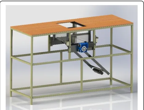
The measurement algorithm is applied to the 3D scan-ning system of foot parameters based on the second-generation Kinect. The scanning system is shown in Fig. 1, and the overall structure consists of the servo motor, high-precision reducer, tension
spring anti-backlash structure, brackets, limit switches, and U-shaped tempered glass. During the measurement, the tester stands on the transparent tempered glass, and the motor drives the long rod to drive the camera around the sole to make a circular motion. The scanning angle is 270°, and the scanning time is 10 s.
2.2 Foot shape 3D reconstruction based on improved ICP algorithm
The first step of the foot shape measurement is to perform image stitching on each frame of depth image captured by the Kinect camera, that is to ro-tate and translate other frame images into the space of the first frame image, let the same physical points coincide and remove noise points. This process is also called point cloud matching.
The stitching of the depth image often adopts the interactive closest points (ICP) algorithm, which was proposed by Besl and Mckay [16] in the 1980s. The process can be expressed as given two depth images sets
P and Q, where pi(xi,yi,zi)∈P(i= 1, 2,…,n) and qj(xj,yj, zj)∈Q(j= 1, 2,…,m). Their Euclidean distance in 3D space is expressed as:
d p!i;q!j
¼!pi;q!j¼
ffiffiffiffiffiffiffiffiffiffiffiffiffiffiffiffiffiffiffiffiffiffiffiffiffiffiffiffiffiffiffiffiffiffiffiffiffiffiffiffiffiffiffiffiffiffiffiffiffiffiffiffiffiffiffiffiffiffiffiffiffiffi
xi−xj
2
þ yi−yj
2
þ zi−zj
2
r
ð1Þ
The purpose of the 3D point cloud matching problem is to find a pair of matrices, including a rotation matrix
R and a translation matrix T. For ! ¼qi R p! þi T, using the least squares method to find the optimal solution to minimize E¼PNi¼1j!qi−ðR!piþTÞj
2
. After k iterations, the corresponding point coordinates of the point cloud
Pafter rotation and translation isQkiði¼1;2;…;nÞ. Cal-culating the rotation and translation matrix between P
and Qki and updating the original matrix until the sum of the Euclidean distances of the point cloudsP andQki
is less than a given thresholdτ.
Each iteration of the ICP algorithm brings the two depth images closer together, and Turk et al. [17] dem-onstrate the convergence of the algorithm. However, when the number of point clouds in the image is large, the calculation amount is large, and the calculation speed is relatively slow. At the same time, the trad-itional ICP algorithm has a small distance per iteration transformation, which is a process of gradually rotating and translating, and the stitching speed is very slow. The number of foot point clouds that need to be proc-essed in this paper is between several hundred thou-sand and several million, and the splicing process is very time-consuming. Therefore, we have optimized
and improved the traditional ICP algorithm for specific application scenarios.
The foot scan system used in this paper has a scan angle of 270° around the foot and lasts for 10 s. The depth image acquisition frame rate is 30 fps, so the rotation angle between each frame image can be cal-culated as:
α¼ Angel
timeframe=second¼ 270
1030¼0:9 ð2Þ
That is, in an ideal case, the adjacent two frames of images are rotated by 0.9° and the translational dis-tance is 0 m. This ideal case means that the rotating speed of the motor is uniform, and the rotating angle between each frame is the same, and there is no gap between the shaft gear of the long rod and the motor gear; the distance between the camera and the foot is always the same during the scanning process. The ideal situation is close to the actual situation, and al-gorithm optimization based on this ideal condition can effectively improve the efficiency of the algorithm. In this ideal case, corresponding to the Z-axis in the 3D space coordinates, the initial rotation matrix T0
and the translation matrix R0 are:
T0¼ cos 0ð :9Þ −sin 0ð :9Þ sin 0ð :9Þ cos 0ð :9Þ
ð3Þ
R0¼0 ð4Þ
Therefore, the improved ICP algorithm process in this paper is as follows:
1) Translate and rotateQ0toM0with the above rotation matricesT0andR0, makingQ=M0. 2) Sample the base point setP, takingPk
i∈P.
3) Take the corresponding point set ofQ, so that Pn
i¼1kPki−Qkik 2
takes the minimum value. 4) Find the rotation matrixRkand the translation
matrixTkto minimizePni¼1kPk
i−ðRkQki þTkÞk 2
. 5) Calculate the average errordkþ1¼1
n
Pn i¼1 kPk
i−Qkiþ1k 2
.
6) Whendk+ 1is greater than the set thresholdτ, return to 2) to iterate, and whendk+ 1<τork>kmax(the
maximum number of iterations set), exit iteration.
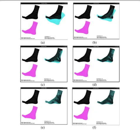
The traditional ICP algorithm and the improved ICP algorithm are used for splicing the foot depth image, as shown in Fig. 2 and Fig. 3. In the single image, the upper left black point cloud is the first frame depth image, and the lower left purple point cloud is the sec-ond frame foot depth image, they are in the same 3D coordinate system but have distances in the horizontal and vertical directions. The stitched picture is shown
on the right side of the figure, wherein the first frame image is not moved as a reference, and the second frame image is rotated and translated by the ICP algo-rithm and superimposed on the reference image. As can be seen from the figure, as the number of iterations increases, the point cloud data of the two foot shapes are gradually spliced together, and the higher the degree of co-incidence, the better the splicing effect. In Fig.2, after 42 iterations, the two foot depth images almost completely coincide. However, in Fig.3, it happened on 32 iterations. It can be seen that the improved ICP algorithm greatly re-duces the number of iterations and improve the speed of image stitching.
Repeating the above experiment 50 times for different two-frame depth images, the traditional ICP algorithm achieves an overlap of 41.3 times on average, and the improved ICP algorithm achieves an overlap of 30.1 times on average, and the stitching speed is increased by 27.1%. The improved ICP algorithm for specific scenes reduces the computational complexity of image stitching and speeds up the real-time reconstruction.
This paper draws on the KinectFusion algorithm framework provided by Microsoft [18] and designs a 3D reconstruction algorithm framework for foot shape. First, the foot is scanned by a self-designed 3D scan-ning system to obtain a depth image of the foot shape. Then, the algorithm provided by KinectFusion is used for denoising and camera parameter calibration, and fi-nally, the 3D reconstruction is completed by the im-proved ICP algorithm.
Figure4a is the result of the 3D scanning using the im-proved ICP algorithm proposed in this paper. It can be seen that the 3D foot shape obtained by the reconstruc-tion algorithm has a smooth overall shape, the details are clear, and the noise is small. Comparing with the results of the DynaScan4D laser scanner in the article by Van den Herrewegen et al. [19], as shown in Fig.4b, it can be seen that the 3D reconstruction of the latter’s foot is rough, and there are gaps in many places. The details of the foot are not obvious enough, and the point cloud distribution is sparse. The smooth 3D reconstruction lays a good foun-dation for the measurement of the 3D foot shape parameters.
2.3 Coordinate transformation
The measurement algorithm of the foot shape feature parameters is closely related to the installation of the camera of Kinect, the trajectory of the camera, and the relative standing position of the tester.
X-axis,Y-axis, and Z-axis, respectively. In actual measure-ment, the position and orientation of the tester cannot be strictly corresponding to the coordinate axis; it is neces-sary to rotate and translate the original 3D foot shape in the coordinate system, so as to make the measurement more convenient.
According to the actual situation of the experimental platform, this paper takes the heel as the starting point. According to the application scenario, the point with the smallest Y-axis value is determined as the heel point, and the point with the largestY-axis value is determined as the toe point.
Set the heel coordinate to O(x0,y0,z0), for each point P(xi,yi,zi)(i= 1, 2, 3,…,n) on the 3D foot point cloud, the coordinates translated to the origin are:
P0ðxi−x0;yi−y0;zi−z0Þði¼1;2;3;…;nÞ:
Next, we translate the foot length rotation to the
Y-axis, which translates the heel and toe points to the
Y-axis. Set the toe point coordinates toP1(x1,y1,z1), then
the angleθ1between the vectorOP1 and the XOY plane
is:
Fig. 2Iteration of traditional ICP algorithmaIteration oncebIteration 5 timescIteration 10 timesdIteration 15 timeseIteration 42 timesf
θ1¼ arctan z1 ffiffiffiffiffiffiffiffiffiffiffiffiffiffiffi x2
1þy21 p
!
ð5Þ
Then, the angleθ2between the vector OP1 and the Y
plane is:
θ2¼ arctan x1 ffiffiffiffiffiffiffiffiffiffiffiffiffiffiffi x2
1þy21 p
!
ð6Þ
Thus, each point cloud coordinate on the 3D foot shape is rotated counterclockwise by the angleθ1with theX-axis
as the rotation axis and theZ-axis is used as the rotation
axis, and the angleθ2is rotated to translate the foot length
direction to theY-axis.
Finally, the largest point in theX-axis direction coordin-ate value is determined as the first metatarsophalangeal inner width point Q1(xq1,yq1,zq1), and the smallest point
in the X-axis direction is the fifth metatarsophalangeal outer width pointQ2(xq2,yq2,zq2). It is necessary to rotate Q1Q2 to be parallel to the XOY plane. When measuring
the 3D foot shape, the plantar plane is parallel to the XOY plane, which ensures that the maximum and minimum points in the X-axis coordinate value correspond to the first metatarsophalangeal inner width point and the fifth metatarsophalangeal outer width point, respectively. The
Fig. 3Iteration of improved ICP algorithmaIteration oncebIteration 5 timescIteration 10 timesdIteration 15 timeseIteration 32 timesf
angle needed to rotate the 3D foot shape along theY-axis is:
θ3¼ arctan
zq2−zq1 xq2−xq1
ð7Þ
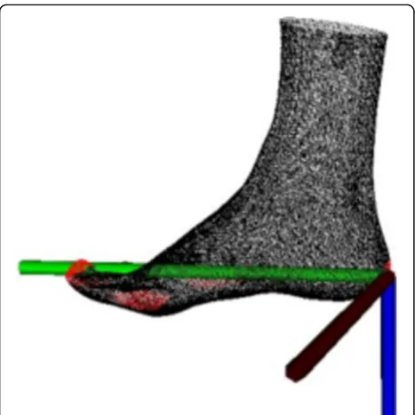
In this way, the rotation and translation of the original 3D scanning foot model to the new spatial coordinate sys-tem have been completed. The final 3D foot shape is based on the heel as the origin, the foot length direction as theY-axis, the foot width direction as theX-axis, and the lower leg direction as the negative Z-axis coordinate system. As shown in Fig. 5, black is the X-axis, green is theY-axis, and blue is theZ-axis. The above work is ready for the measurement of 3D foot shape feature parameters.
3 Method: 3D foot shape feature parameters measurement
3.1 Measurements of foot length and width
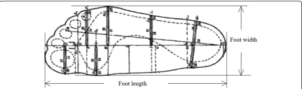
In the National Standards of China [20], foot parameters are defined as shown in Fig.6. The foot length is defined as the distance between the second phalanx and the heel, and the foot width is defined as the horizontal distance between the first metatarsophalangeal inner width point and the fifth metatarsophalangeal outer width point.
In this paper, foot length and foot width are measured according to the standards mentioned above and also maintains the standard in the following manual meas-urement process.
Set toe point 3D coordinate toP1(x1,y1,z1), so the foot
length measurement formula is:
footlength¼y1 ð8Þ
Since the 3D coordinates of the first metatarsophalan-geal inner width point isQ1(xq1,yq1,zq1), the 3D
coordi-nates of the fifth metatarsophalangeal outer width point is Q2(xq2,yq2,zq2). We can see that the foot width
meas-urement formula is:
footwidth¼xq1−xq2 ð9Þ
3.2 Measurements of metatarsale girth
The length of metatarsale girth is the length of making a complete circle around the foot [21]. In this paper, we define the metatarsale girth as the length of the inter-secting line of the foot and the plane which is perpen-dicular to the XOY plane and passes through the first metatarsophalangeal inner width point and the fifth metatarsophalangeal outer width point. Which is to say, the intersection line is formed by the intersection of the 3D foot shape and the plane which is perpendicular to the horizontal direction and passes through the first metatarsophalangeal inner width point Q1(xq1,yq1,zq1)
and the fifth metatarsophalangeal outer width point
Fig. 4Comparison of 3D reconstruction effect of foot shape
Q2(xq2,yq2,zq2). The intersection line has the following
characteristics:
1) Composed of point clouds. The intersection line consists of 3D point clouds since theY-axis coordinates of these points are the same; the perimeter of the 3D point clouds can be reduced to the perimeter of the 2D point, which can be solved by a 2D plane algorithm.
2) Irregular. The physical characteristics of the foot determine that the perimeter is irregular. 3) Closed. The usual curve fittings are open curves,
but the metatarsale girth is a closed curve, connected end to end.
4) Smooth. Although each person’s foot shape is different, they are all smooth.
Different from the traditional method of using a high-order polynomial function to fit a closed curve, we use the B-spline curve fitting algorithm [22] to calculate, which is suitable for fitting dense point clouds data [23,24]. The B-spline curve is composed of segmented spline curves. Each curve is controlled by a polygon composed of specific control points, which can de-scribe the characteristics of the object locally without affecting the global fitting [25]. At the same time, the curve is more free and smooth, and the fitting effect is better.
B-spline is a kind of function; it is defined as a piece-wise polynomial, given a vector combination of intervals [a, b],Δ:a=x0<x1<…<xn=b. If function g(x) satisfies (1) on vector [xi,xi+ 1], g(x) is a k-degree polynomial of x; (2)g(x)∈Ck−1[a,b], that is, g(x) has a continuous k−
1 order derivative on [a, b]. Then, we call g(x) as a
k-spline function for vector combinationΔon [a,b] and
xi(i= 0, 1,…,n) as a control point for B-spline. For a set of control point combinations, all ktimes splines make up one spatial combination, calledk-spline space [26].
A group of basis functions ink-degree spline space is called k-degree B-spline basis function. For the vector combination T:ftig∞t¼−∞;ti≤tiþ1;i¼0;1;… on the t-axis, the functionNi, k(t) defined by the following for-mula recursively is called the k−1 order B-spline basis function for the vector combinationT:
Ni;1ð Þ ¼t 10;;otherwiset∈½ti;tiþ1Þ
Ni;kð Þ ¼t
t−ti
tiþk−1−ti
Ni;k−1ð Þ þt tiþk−t
tiþk−tiþ1
Niþ1;k−1ð Þt ;k≥2
0
0¼0
8 > > > > > < > > > > > :
ð10Þ
This formula is called the de Boor-Cox formula [27]. WhereT is called the control point sequence or control point vector, and ti is called the control point. It is ex-tracted during the fitting process.
When point cloudsQ= {qj:j= 1, 2,…r} is in a B-spline curve, the following formula should be satisfied [28]:
qj uj ¼
Xn
j¼0
Nj;P uj Pj;j¼1;2;…r ð11Þ
In Eq. 11, the matrix can be simply written asQ=NP, and Q is composed of r × 3 matrices of r point clouds data, N is composed of r × n B-spline basis function co-efficient matrices, and P is controlled by n control verti-ces which are composed of n × 3 matrices. If the point clouds Q are parameterized and then the control point vector of the curve is divided, then the basis function coefficient matrix N is obtained, so that the control ver-tices P are determined. In summary, the process can be summarized as follows: by the points that falling on the curve or lying around the curve, the parameters related to the curve can be pushed back to obtain and then the B-spline curve can be determined.
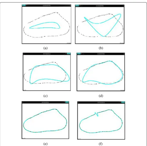
Fig. 7B-spline curve fitting processaControl points 3bControl points 4cControl points 5dControl points 15eControl points 40fControl points 80
Table 1The relationship between the number of control points and the length of the metatarsale girth
Control point 3 4 5 6 7 8 9 10 11
Plantar circumference(cm) 13.37 13.37 13.37 13.37 20.19 22.83 21.81 22.74 22.61
Control point 12 13 14 15 17 20 25 30 35
Plantar circumference(cm) 22.79 22.94 22.98 23.01 23.16 23.21 23.25 23.27 23.30
Control point 40 45 50 55 60 65 70 75 80
In the 3D foot shape model, we save the point clouds of the intersection line of the foot and the plane which is per-pendicular to the XOY plane and passes through the first metatarsophalangeal inner width point and the fifth meta-tarsophalangeal outer width point. As the point cloud on the interception surface is sparse, it is considered that the point cloud within a distance of 0.01 mm from the inter-ception plane is the point cloud on the intersection line, and theY-axis coordinates are determined to be the same; then, the curve in 3D space can be transformed into 2D space to facilitate the solution of the perimeter of the curve. The point clouds data of the metatarsale girth is fitted by B-spline curve fitting algorithm. Through constrain-ing the control points multiple times, in the case of dif-ferent numbers of control points, the effect of difdif-ferent curve fitting is as follows:
We have carried out multiple fittings. The length of the metatarsale girth we obtained in the case of different control points is shown in Table1:
As can be seen in Fig. 7, when the number of control points is small, the fitted curve is relatively simple and rough, which does not coincide well with the fitted point clouds, and some may even be deformed, making the fit-ted curve deviate further from the point cloud. When the number of control points reaches about 40, the curve can express the contour of the point clouds well. At the same time, the curve is even and smooth, and the local features can also be well fitted. The point cloud ba-sically falls on the fitting curve. When the control points are relatively large, such as 80, overfitting occurs locally, and the curve is not smooth enough and deformed, which does not meet the physical characteristics of the foot. From the above experiment and analysis, the num-ber of control points for the B-spline curve fitting in this paper was selected as 40. At this time, the fitting was smooth and the details of the metatarsale girth were highlighted.
4 Experiment results and discussions
The experimental process is shown in Fig.8. The tester stood barefooted on the transparent tempered glass. The motor drove a long rod and drove the camera rotating around the sole to make a circular motion. The scanning angle was 270°, and the scanning time was 10 s.
4.1 System stability
The foot shape of the same subject was measured ten times. The foot length and the length of the metatarsale girth were automatically determined for each of the right and left foot. Table2 shows the result of the foot shape parameters being measured.
Calculate the mean squared error of the ten groups of data measurement results. For foot length data, the left foot has a variance of 0.1 mm and the right foot has a
variance of 0.2 mm. For the metatarsale girth data, the left foot has a variance of 0.3 mm and the right foot has a variance of 0.3 mm.
From the above results, it can be seen that the mean squared error of each measurement is small, and the consistency of the measurement results is good, indicat-ing that the system based on this algorithm has high measurement stability.
4.2 System accuracy
3D foot shape measurement system was used to measure 3D foot shape images of 20 subjects, and the parameters such as their foot length and metatarsale girth were lated based on the algorithm. The mean value was calcu-lated three times. At the same time, we used a tape measure to manually measure the parameters such as the
Fig. 8The experimental process of 3D foot shape scanning system
Table 2Result of multiple measurements of foot length and
metatarsale girth
Foot length Plantar circumference
Left (cm) Right (cm) Left (cm) Right (cm)
1 26.1 26.2 25.4 25.1
2 26.2 25.8 24.8 24.7
3 26.5 25.9 25.2 25.2
4 26.3 25.9 25.1 25.2
5 26.1 26.2 25.4 25.1
6 26.4 26.1 25.0 25.2
7 26.3 26.2 25.3 25.0
8 26.4 26.0 24.8 24.8
9 26.2 25.8 25.3 24.7
10 26.3 26.1 25.0 24.9
length of the foot and the metatarsale girth of the testers; the same measurement was performed three times to ob-tain the average value. Manual measurement is strictly carried out in accordance with the definitions of foot length, foot width, and plantar circumference in the na-tional standards and references. The differences between the two data are compared, as shown in Table3:
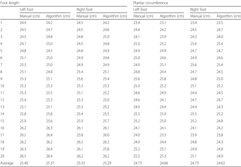
From Table3, it can be seen that for the measurement of the foot length, the maximum error is 3.0 mm and the average error is 0.35 mm. For the measurement of the plantar circumference, the maximum error is 5.0 mm and the average error is 0.85 mm. It can be seen that the measurement system using our proposed algo-rithm has an average error of less than 0.85 mm com-pared to the manual measurement. The error value is smaller than the foot’s difference in sensitivity (the shoe last size difference that people can feel, generally 6 mm for men and 2.08 mm for women), which can meet the needs of customized shoemaking.
Comparing our system with the laser foot scanner LSF-390 of Stereo3D Technology Co., Ltd., China, IDEAS company’s FootScanner FTS-4© and the CCD camera 3D scanning scheme of Zhejiang University, China, as shown in Table4.
Based on Kinect 2 scan system, this paper designs a matching algorithm for measuring foot shape parame-ters. It can be seen from the table that our system can measure the parameters of both feet at the same time, which greatly simplifies the scanning process. The sys-tem is not affected by ambient light and greatly reduces the manufacturing cost of the scanning system.
Table 4Comparison table with other scanning system
parameters
LSF-390 FootScanner FTS-4
CCD camera 3D scanning scheme
Ours
Company or institution
Stereo3D Technology Co.
IDEAS S.A. Zhejiang University, China
–
Precision (mm) 0.5 0.5 1 1
Time for single measurement (s)
10 1 1 10
Number of feet once measured
1 1 1 2
Cost (thousand dollars)
30 15 2 0.8
Ambient light effect
Greatly Large Greatly Small
Table 3Comparison of the results of the measurement algorithms and manual measurement
Foot length Plantar circumference
Left foot Right foot Left foot Right foot
Manual (cm) Algorithm (cm) Manual (cm) Algorithm (cm) Manual (cm) Algorithm (cm) Manual (cm) Algorithm (cm)
1 24.4 24.2 24.5 24.2 23.4 23.1 23.4 23.5
2 24.5 24.7 24.5 24.6 24.4 24.2 24.5 24.7
3 24.5 24.8 24.8 25.0 24.1 23.9 24.3 24.0
4 24.7 25.0 24.5 24.8 25.0 25.2 25.6 25.4
5 24.8 24.5 24.8 24.9 24.9 24.9 24.7 24.7
6 25.1 25.0 24.9 24.6 25.0 24.6 24.9 24.6
7 25.3 25.0 24.9 24.9 24.9 25.1 25.6 25.4
8 25.1 24.8 25.4 25.1 24.8 24.4 24.7 24.5
9 25.3 25.1 25.6 25.4 25.6 25.8 24.8 25.0
10 25.3 25.3 25.3 25.3 25.0 25.2 25.1 25.2
11 25.3 25.5 25.1 25.2 24.6 24.9 24.4 24.5
12 25.4 25.3 25.3 25.0 24.6 24.1 24.7 24.7
13 25.1 25.1 25.3 25.2 24.0 24.4 24.4 24.3
14 25.8 25.8 25.4 25.5 25.5 25.9 25.5 25.2
15 25.9 25.6 25.9 25.7 25.2 25.0 25.2 24.8
16 26.2 26.3 26.1 26.1 24.1 24.1 24.1 24.2
17 26.2 26.4 25.8 26.0 24.0 23.5 23.9 23.8
18 26.2 26.2 26.2 26.2 24.9 24.4 24.8 24.3
19 26.3 26.4 26.1 25.8 25.2 25.1 24.9 24.8
20 26.5 26.4 26.2 26.2 25.3 25.3 25.1 24.9
Although the scanning accuracy and acquisition time index of this system are not the best, it has fully met the application requirements. In contrast, the system is a preferred solution for the foot scanning application.
5 Conclusion
Based on the 3D foot shape acquisition system based on second-generation Kinect, a 3D foot shape feature par-ameter measurement algorithm is proposed. The most important parameters such as foot length, foot width, and metatarsale girth are measured. The consistency of the measurement system based on the algorithms is bet-ter, and the error of the foot shape parameters obtained by manual measurement is smaller, which can meet the needs of customized shoemaking and lay a good founda-tion for the automafounda-tion and standardizafounda-tion of custom-ized shoemaking.
In the following work, we will increase the number of experimental samples and improve the measurement al-gorithms based on the measured big data to further im-prove the foot shape measurement accuracy.
Abbreviation
CCD:Charge-coupled device
Acknowledgements
The authors thank the editor and anonymous reviewers for their helpful comments and valuable suggestions.
Funding
The project has been supported by the special fund for the development of Shenzhen(China) strategic new industry (JCYJ20170818085946418) and the Shenzhen (China) Science and Technology Research and Development Fund (JCYJ20170306092000960).
Availability of data and materials
We can provide the data.
Authors’contributions
MW completed the coordinate transformation of the system and the processing and analysis of the 3D point cloud data. XAW provides guidance in the implementation of the project. ZCF and SXZ carried out the collection and screening of the experimental data and preprocessed the data. CP and ZL completed the construction and the test of the hardware system. All authors read and approved the final manuscript.
Authors’information
Mo Wang received the B.S. degree in Electronic Science and Engineering from Jilin University, Jilin, China, in 2011. From 2012 to now, he is pursuing the Ph.D. degree in the school of electronic and computer engineering in Peking University Shenzhen Graduate School, Guangdong, China. His interests include 3D image processing and human motion information collection based on multi-sensors.
Xin’an Wang received the B.S. degree in Computer Science from Wuhan University, Wuhan, China, in 1983, and the M.S. and Ph.D. degrees in Microelectronics from Shanxi Microelectronics Institute, Xi’an, China, in 1989 and 1992, respectively. He is currently a Professor at the School of Electronics Engineering and Computer Science, Peking University Shenzhen Graduate School, Beijing, China. He is currently with the School of Electronic and Computer Engineering, Peking University, Shenzhen Campus. His research interests are focused on monitoring on human body movement and life health.
Zhuochen Fan received the B.S. degree in College of Communications Engineering at Chongqing University in 2017. He is currently a graduate student in the school of electronic and computer engineering in Peking
University Shenzhen Graduate School, Guangdong, China. His interests include 3D image processing.
Sixu Zhang received the B.S. degree in Electronic Science and Engineering from Jilin University, Jilin, China, in 2017. He is currently a graduate student in the school of electronic and computer engineering in Peking University Shenzhen Graduate School, Guangdong, China. His interests include 3D image processing and modeling.
Chen Peng received the B.S. degree in College of Electronic Science and Applied Physics from Hefei University of Technology, Anhui, China, in 2017. He is currently a graduate student in the school of electronic and computer engineering in Peking University Shenzhen Graduate School, Guangdong, China. His interests include automatic control.
Zhong Liu received the B.S. degree in School of Physics at Sun Yat-sen Uni-versity in Guangdong, China, in 2017. He is currently a graduate student in the school of electronic and computer engineering in Peking University Shenzhen Graduate School, Guangdong, China. His interests include intelli-gent human motion information collection.
Competing interests
The authors declare that they have no competing interests.
Publisher’s Note
Springer Nature remains neutral with regard to jurisdictional claims in published maps and institutional affiliations.
Received: 11 August 2018 Accepted: 23 October 2018
References
1. R.T. Lewinson et al., Foot structure and knee joint kinetics during walking with and without wedged footwear insoles. J. Biomech.73, 192–200 (2018) 2. R. Molfino, M. Zoppi, Mass customized shoe production: a highly
reconfigurable robotic device for handling limp material. Robot. Autom. Mag. IEEE12(2), 66–76 (2005)
3. X. Shuping et al., Foot measurements from 2D digital images. IEEE Int Conf Ind Eng Eng Manag IEEE, 497–501 (2010).https://doi.org/10.1109/IEEM.2010. 5674498
4. T. Nagamatsu et al., User-calibration-free gaze estimation method using a binocular 3D eye model. Ieice Trans.Inf. Syst.94(9), 1817–1829 (2011) 5. M. Maruyama, S. Tabata, Y. Watanabe, Multi-pattern embedded phase
shifting using a high-speed projector for fast and accurate dynamic 3D measurement. IEEE Wint. Conf. Appl. Comp. Vis. IEEE. Comp. Soc., 921–929 (2018).https://doi.org/10.1109/WACV.2018.00106
6. P. Psota et al., Surface profilometry by digital holography. IEEE Int. Conf. Emerg. Technol. Fact. Autom. IEEE, 1–5 (2017).https://doi.org/10.1109/ETFA. 2017.8247748
7. I. Pioaru, Visualizing virtual reality imagery through digital holography. Int. Conf. Cyberworlds, 241–244 (2017).https://doi.org/10.1109/CW.2017.50 8. S. Wang et al., Accurate and robust surface measurement using optimal
structured light tracking method. Ieice Trans.Inf. Syst93(2), 293–299 (2010) 9. B. Novak, J. Možina, M. Jezeršek, 3D laser measurements of bare and shod
feet during walking. Gait Posture40(1), 87–93 (2014)
10. M. Jezersek, J. Mozina, High-speed measurement of foot shape based on multiple-laser-plane triangulation. Opt. Eng.48(11), 933–956 (2009) 11. Lee, Hyunglae, K. Lee, and T. Choi. Development of a low cost foot-scanner for
a custom shoe tailoring system. Symposium on Footwear Biomechanics (2005) 12. FootScanner FTS-4. [EB/OL].http://www.ideas.be/Default.aspx?tabid=263.
Accessed 20 June 2018
13. F. Gao, Q. Wang, W.D. Di, et al., Acquisition of time-varying 3D foot shape from video. Sci China Press41(6), 659–674 (2011) (in Chinese)
14. 3D foot scanner LSF390. [EB/OL].http://www.3doe.com/en/ggggg/124-38. html. Accessed 20 June 2018
15. Y.W. Song, Z.X. Wang, Y. Su,The principles of footwear biomechanics and
application(China Textile and Apparel Press, Beijing, 2014) (in Chinese)
16. P.J. Besl, N.D. Mckay, Method for registration of 3-D shapes. IEEE Trans. Pattern Anal. Mach. Intell.14(2), 239–256 (2002)
17. Turk et al., Zippered polygon meshes from range images. Comput. Graph., 311–318 (1994).https://doi.org/10.1145/192161.192241
19. H. Van den I et al., Dynamic 3D scanning as a markerless method to calculate multi-segment foot kinematics during stance phase: methodology and first application. J. Biomech.47(11), 2531–2539 (2014)
20. J.Q. Wang, X. Zhou, Z.M. Yao, Design and implementation of the foot parameter measurement system based on computer vision. Instrum. Technol.7, 40–44 (2012) (in Chinese)
21. Y. Song, B. Xu, N. Shen, Research on measurement angles of three dimensional foot type. Chin. Leather42(16), 119–121 (2013) (in Chinese) 22. Z. Wu et al., Fitting scattered data points with ball B-spline curves using
particle swarm optimization. Comput. Graph.72, 1–11 (2018)
23. L.A. Piegl, W. Tiller, Least-squares B-spline curve approximation with arbitary end derivatives. Eng. Comput.16(2), 109–116 (2000)
24. J.S. Kim, S.M. Choi, Interactive cosmetic makeup of a 3D point-based face model. Ieice Trans.Inf. & Syst 916, 1673–1680 (2008)
25. J. Yang et al., The application of evolutionary algorithm in B-spline curved surface fitting. Int. Conf. Artif. Intell. Comput. Intell. Springer-Verlag, 247–254 (2012).https://doi.org/10.1109/FSKD.2012.6234112
26. J.L. Han,Multi-degree B-spline curves(Zhejiang University, Hangzhou, 2007) (in Chinese)
27. H. Yang et al., The deduction of coefficient matrix for cubic non-uniform B-spline curves. Int. Workshop Educ. Technol. Comput. Sci. IEEE, 607–609 (2009).https://doi.org/10.1109/ETCS.2009.396