On the use of watermark-based schemes to detect cyber-physical attacks

R E S E A R C H

Open Access

On the use of watermark-based schemes

to detect cyber-physical attacks

Jose Rubio-Hernan

, Luca De Cicco

and Joaquin Garcia-Alfaro

Abstract

We address security issues in cyber-physical systems (CPSs). We focus on the detection of attacks against cyber-physical systems. Attacks against these systems shall be handled both in terms of safety and security.

Networked-control technologies imposed by industrial standards already cover the safety dimension. However, from a security standpoint, using only cyber information to analyze the security of a cyber-physical system is not enough, since the physical malicious actions that can threaten the correct behavior of the systems are ignored. For this reason, the systems have to be protected from threats to their cyber and physical layers. Some authors have handled replay and integrity attacks using, for example, physical attestation to validate the cyber process and to detect the attacks, or watermark-based detectors which uses also physical parameters to ensure the cyber layers.

We reexamine the effectiveness of a stationary watermark-based detector. We show that this approach only detects adversaries that do not attempt to get any knowledge about the system dynamics. We analyze the detection ratio of the original design under the presence of new adversaries that are able to infer the system dynamics and are able to evade the detector with high frequency. We propose a new detection scheme which employs several non-stationary watermarks. We validate the detection efficiency of the new strategy via numeric simulations and via running experiments on a laboratory testbed. Results show that the proposed strategy is able to detect adversaries using non-parametric methods, but it is not equally effective against adversaries using parametric identification methods.

Keywords: Cyber-physical security, Control theory, Network security, Networked-control system, Critical infrastructures, Attack detection, Adversary model, Cyber-physical adversary, Attack mitigation

1 Introduction

In an effort to reduce complexity and costs, tradi-tional industrial control systems are being upgraded with novel computing, communication, and interconnection capabilities. Industrial control systems that close the loop through a communication network are hereinafter referred to ascyber-physical systems. The adoption of new communication capabilities comes at the cost of introduc-ing new security threats that are required to be holistically handled, both in terms of safety and security (in the tra-ditional ICT sense). The recently coined cyber-physical securityterm refers to the mechanisms that address this specific challenge [1].

The use of inadequate cyber-physical security mecha-nisms may have an adverse effect on a vast number of

*Correspondence: [email protected] 1_{SAMOVAR, Telecom SudParis, CNRS, Université Paris-Saclay, 9 Rue Charles} Fourier, 91000, Evry, France

Full list of author information is available at the end of the article

resources, including assets of private companies, govern-ment networks, and mission critical infrastructures [2]. The associated costs, especially in terms of loss of business opportunities and the expenses for fixing the incidents, are expected to be reduced. As a consequence, the issue of the assessment of cyber-physical security mechanisms is a hot research topic.

In this paper, we address security in industrial control systems. Our focus is centered on integrity issues due to the interconnection betweencyber andphysical control domains in networked-control systems. More specifically, we focus on the adaptation of physical-layer failure detec-tion mechanisms (e.g., systems for the detecdetec-tion of faults and accidents) to handle, as well as, attacks (e.g., replay and integrity attacks conducted by malicious adversaries). We extend the work proposed in [3] which reexamines the security of a specific scheme proposed by Mo et al. in [4, 5].

The Mo et al. scheme relies on the adaptation of a real-time failure detector based on alinear time-invariant

model of the system. Built upon Kalman filters and linear-quadratic regulators, the scheme produces authentication watermarks to protect the integrity of physical measure-ments communicated over the cyber and physical con-trol domains of a networked-concon-trol system. Without the protection of the messages, malicious actions can be con-ducted to mislead the system toward unauthorized or improper actions and affect the availability of the system services.

We show that the Mo et al. detection scheme only works against some integrity attacks. We present two adver-sary models that can evade the Mo et al. detector. These adversaries are classified based on the algorithm used to obtain the knowledge of the system dynamics in order to carry out the attack (non-parametric [3] and parametric adversaries [6]).

Contributions The main contributions of this paper are summarized as follows:

• We reexamine the effectiveness of the attack detector proposed in [4, 5] under new adversary models. • We show detection weaknesses in [4, 5] under the

new adversary models.

• Enhanced detector approaches against the new adversaries are presented and validated via numerical simulations and experiments carried out by using a real testbed.

Paper organization Section 2 provides the necessary background for the paper. Section 3 reviews the detector scheme in [4, 5], and defines our adversary models and reexamines the security of the detector under the new adversary models. Section 4 adapts the detection scheme in [4, 5] to handle the uncovered limitations and vali-dates the resulting approach via numerical simulations. Section 5 presents experimental results based on a labo-ratory testbed. Section 6 discusses the results. Section 7 reviews some related work. Section 8 concludes the paper.

2 Background

2.1 Industrial control systems

We assume Industrial Control Systems built upon Super-visory Control and Data Acquisition (SCADA) technolo-gies and Industrial Control Protocols. Such combinations are hereinafter denoted as networked-control systems. Some more information about these systems and proto-cols follows.

2.1.1 SCADA

General term that encompasses well-defined types of field devices, such as: (1) master terminal units (MTUs)

and Human Machine Interfaces (HMIs), located at the topmost layer and managing all communications; (2) remote terminal units (RTUs), and programmable logic controllers (PLCs), controlling and acquiring data from remote equipment and connecting with the master sta-tions; (3) sensors and actuators.

The MTUs of a SCADA system are located at the con-trol center of the organization. The MTUs give access to the management of communications, collection of data (generated by several RTUs), data storage, and control of sensors and actuators connected to RTUs. The interface to the administrators is provided via the HMIs.

RTUs are stand-alone data acquisition and control units. They are generally microprocessor-based devices that monitor and control the industrial equipment at the remote site. Their tasks are twofold: (1) to control and acquire data from process equipment (at the remote sites), and (2) to communicate the collected data to a master (supervision) station. Modern RTUs may also communi-cate between them (either via wired or wireless networks). PLCs are small industrial microprocessor-based com-puters. Most significant differences with respect to an RTU are in size and capability. An RTU has more inputs and outputs than a PLC, and much more local processing power (e.g., to postprocess the collected data before gen-erating alerts toward the MTU via the HMI). In contrast, PLCs are often represented by pervasive sensors with communication capabilities. PLCs have two main advan-tages over traditional RTUs: (1) they are general-purpose devices enforcing a large variety of functions, and (2) they are physically compact.

Sensors are monitoring devices responsible for retriev-ing measurement related to specific physical phenomena and feed them to the controller. Sensors typically convert a measured quantity to an electrical signal, which is later converted and stored as data. Sensors can be seen as the input function of a SCADA system. The data produced by sensors are sent to the upper layers via the RTUs and the PLCs. Finally,actuatorsare control devices, in charge of managing some external devices. Actuators translate control signals to actions that are needed to correct the dynamics of the system, via the RTUs and the PLCs.

2.1.2 Industrial control protocols

Protocols for industrial control systems must cover reg-ulation rules such as delays and faults [7]. However, few protocols imposed by industrial standards provide secu-rity features in the traditional ICT secusecu-rity sense (e.g., confidentiality, integrity, etc.). Details about such ICT security capabilities of representative protocols follows.

probably due to its simplicity and its free license. The Modbus protocol was initially conceived for serial com-munications. Since 1999, it has been adapted to work over TCP/IP as well. The use of Modbus over TCP/IP allows using SCADA components in heterogeneous environ-ments (i.e., working over IP or serial networks). Moreover, it is possible to use gateways to convert Modbus/TCP to serial Modbus.

From a security standpoint, Modbus does not integrate traditional ICT protection features. For instance, in terms of availability, Modbus/TCP may use some function codes (e.g., ECO4: Server Failure, EC06: Server Busy) as the response of a query from an unavailability device. This way, a controller can point out to availability issues in the absence of responses from one or several devices, or if their responses are error codes. Error in handling is per-formed at the application layer. The availability of a given equipment is also related to the implementation of the lay-ers below Modbus (e.g., TCP/IP laylay-ers) and the nature of the media shared for the exchange of data.

The integrity of a Modbus message is validated by using the TCP layer for Modbus/TCP or by adding a control field (cyclic redundancy check or CRC) for Mod-bus/Serial. Nevertheless, without authentication of the message, malicious actions can modify the message and recalculate valid CRCs. This kind of validation must be seen only as a protection against transmission errors. Malicious modification of registers, e.g., time windows, is complex but possible. Replay attacks and, in general, integrity attacks, are also possible.

Finally, the Modbus protocol does not implement encryption of messages. Nevertheless, it is possible to implement encryption by encapsulating Modbus/TCP messages under TLS or IPsec tunnels. Confidentiality is not considered as a crucial property in industrial environ-ments. The deployment of encryption solutions can be seen as detrimental given their complexity (e.g., public key infrastructures, manual deployment of keys, etc.), since it may induce to unnecessary latency delays.

PROFINET Suite of industrial protocols operating at dif-ferent network layers, mainly used in Siemens products. For instance, PROFINET IO is an Ethernet-based pro-tocol associated to the PROFINET suite. Implemented over TCP/IP layers, it allows real-time communica-tion and self-configuracommunica-tion. All equipment implement-ing PROFINET IO must be certified by the PROFIBUS organization. This certification monitors compliance of software, data models, and integrity in a PROFINET environment.

In 1999, the first security extension of PROFINET was released. Referred to as PROFIsafe, it leverages from PROFINET IO, acting as one of its upper layers. This

allows its deployment over less secure networks maintain-ing acceptable error rate such as IEEE 802.11 and IEEE 802.15.1 standards, while ensuring high availability and backwards compatibility for legacy equipment. Legacy operations can yet use the standard layer, called Black channel, while other operations requiring safety proper-ties, can use the new layers. Those new layers include elements such as continuity control, acknowledgment timeouts, peer authentication, integrity check CRCs, etc.

Åkerberg ans Björkman uncovered in [8] some flaws in the protocol routines associated with the generation of CRCs. Indeed, PROFIsafe meet standards where inten-tional attacks are not considered a risk. The protocol does not integrate cryptographic features. It only consid-ers protection to cover from unintentional faults. It should not be considered a protection layer against cyber attacks. Indeed, the PROFINET Safety Guide [9] indicates the use of VPNs whenever ICT security is required. It is important to emphasize that PROFIsafe has been designed to ensure safety and malfunction (e.g., transmis-sion errors). However, it does not ensure security against intentional malicious acts.

DNP3 Short for Distributed Network Protocol version 3, DNP3 is a modern SCADA protocol that includes secu-rity extensions, often referred to as DNP3-SA (DNP3 Secure Authentication). DNP3-SA adds features to DNP3 such as protection against replay attacks by ensuring mes-sage integrity and authentication. The new features are implemented as new function codes of the original DNP3 protocol. In other words, they are defined at upper layers of the original DNP3 protocol suite, without modifying previous function codes, so that all legacy monitoring and diagnostic tools for DNP3 are still valid. This way, DNP3-SA is compatible with legacy devices that do not require from security support.

The DNP3-SA extensions are expected to be highly scalable. They shall allow changing the security algo-rithms, keys sizes, and other parameters to meet future conditions of state-of-the-art installations. Nevertheless, both DNP3 and DNP3-SA are relatively complex proto-cols. The DNP3-SA extensions are relatively young, and the first DNP3-SA products may present vulnerabilities. They do not provide protection against confidentiality attacks either. For the time being, DNP3-SA has not been largely deployed. Given the pace of industrial systems (whose upgrades are often superior to decades), it may take quite long before DNP3-SA is fully tested over large environments.

of CIP (Common Industrial Protocol) over standard Eth-ernet frames [10]. According to [11], EthEth-ernet/IP was the most widely deployed protocol on industrial environ-ments in 2009, with about 30% of active nodes (about 5 million nodes).

Communications over Ethernet/IP can either be in an unconnected mode, using TCP/IP in a client/server model, or they can be in connected mode. In that case, resources are reserved to create a link between two users; UDP/IP and multicast transmissions are employed to make latency as small as possible to enforce real-time con-straints. In fact, Ethernet/IP inherits from Ethernet all its security issues. Moreover, Ethernet/IP environments mainly use UDP/IP connections, and rarely use security mechanisms (in a traditional ICT sense), due to per-formance and real-time constraints [12]. CIP does not implement security features either. Thus, we can con-sider some concerns such as message hijacking, disclosure of communication and configuration details, injection of unauthorized frames, etc.

2.1.3 Networked-control systems (NCSs)

NCSs are spatially distributed systems whose control loops are connected through communication networks. The communication network connects the different com-ponents of a traditional control system, i.e., the controller, sensors, and actuators. Examples include smart grids, smart vehicles, and water distribution systems. The use of a communication network to connect the different components of a control system adds more flexibility in the system and reduces the implementation cost of new installations. However, the use of a communication net-work to decentralize traditional control systems comes at the price of an increased control design complexity. For instance, the analysis and design of the overall system has also to deal with new theoretical challenges due to, for instance, loss of measurements and time-varying sam-pling [13]. The integration of the control system (often referred as physical-space) with the communication net-work (cyber-space) creates a new degree of interaction between these two domains [14].

Communication protocols used in traditional control systems are required to comply with the constrains imposed by industrial standards (e.g., to cover regula-tion roles such as delay and faults). Indeed, prominent industrial control protocols (e.g., Modbus, PROFINET, and Ethernet/IP) are not designed to provide security from a traditional information or network perspective. However, current NCSs use these protocols over TCP/IP or UDP/IP communications (e.g., Modbus over TCP, PROFINET over TCP, and Ethernet/IP over TCP or UDP). Although such combinations can provide some security elements at either their transport or network layers, this is not enough to ensure control-data protection. At the

same time, traditional control systems come with already existing mechanisms to handle failures. Such mecha-nisms are expected to detect faults and avoid accidents. Nevertheless, classical mechanisms conceived to detect failures in control systems are not able to detect inten-tional actions from malicious adversaries holding enough knowledge about the systems. Cryptography can be used to ensure the integrity of control-data. This may partially solve the aforementioned problem. Without underesti-mating cryptographic solutions, in this paper, we consider a complementary solution proposed by Mo et al. [4, 5] to protect the integrity of the physical sensor measurements by means of authentication watermarks. Such watermarks are enforced by adapting a real-time failure detector based on linear time invariant models of industrial control sys-tems. This security solution allows to improve system security in cases where, e.g., cyber-adversaries bypass security measures at upper protocol layers. We present some representative examples in the following section.

2.2 Cyber-physical attacks

The use of communication networks and IT components in traditional control systems paves the way to new vulner-ability issues. The attacks against these setups are named cyber-physical attacks. These threats may target physical processes through the network. In [15], Texeira et al. pro-pose a taxonomy of cyber-physical attacks based on the resources of the adversaries. Such resources are mainly measured in terms of adversary knowledge (e.g., a pri-ori knowledge of the adversary about the system and its security measures). Indeed, the knowledge of the adver-sary about the system is the main resource in order to build up complex attacks, as well as to make them unde-tectable. Based on the degree of the adversary knowledge, the attacks may succeed at violating system properties, such as availability and integrity, as well as to obtaining operational information about the system to make the attacks undetectable.

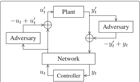
Figure 1 shows an adversary conducting a cyber-physical attack. Thesymbol in the figure represents a

Fig. 1Sample representation of a cyber-physical attack against a networked-control system

Adversaries conducting more powerful injection attacks are expected to modify some of the plant measurements, either by targeting the individual sensors or their com-munication channels in case of insecure communica-tion protocols. Sophisticated variacommunica-tion of the attack in Fig. 1 includes (1) bias-injection cyber-physical attacks, in which the new data injected by the adversary corre-sponds to a bias from the legitimate data, with the aim of leading the system to wrong control decisions (e.g., to cause malfunction in the long-term); and (2) geometric-injection cyber-physical attacks, in which the bias is grad-ually injected. The attack may remain undetected when data compatible with the system dynamics are injected, potentially leading the system to irreversible damages [15]. Another undetectable attack is the covert attack, where the adversary knows perfectly the system model. This attack is defined in [16], and the author concludes that it is not possible to be detected.

Techniques to prevent the aforementioned cyber-physical attacks exist. In [17], Arvani et al. describe a signal-based detector method, using discrete wavelet transformations. Do et al. study in [18] strategies for handling cyber-physical attacks using statistical detec-tion methods. Mo et al. propose in [4, 5] the use of watermark-based detection by adapting traditional fail-ure detection mechanisms (e.g., detectors to handle faults and errors). In the following sections, we elaborate further on the watermark-based technique by Mo et al. discuss about some security limitations and propose an improved technique.

3 Watermark-based attack detection

In [4, 5], a watermark-based strategy is proposed to detect replay and injection attacks against cyber-physical sys-tems. This section reviews the mechanism proposed in [4, 5] and assesses its performance when a new adver-sary model, that we name cyber-physical adversary, is

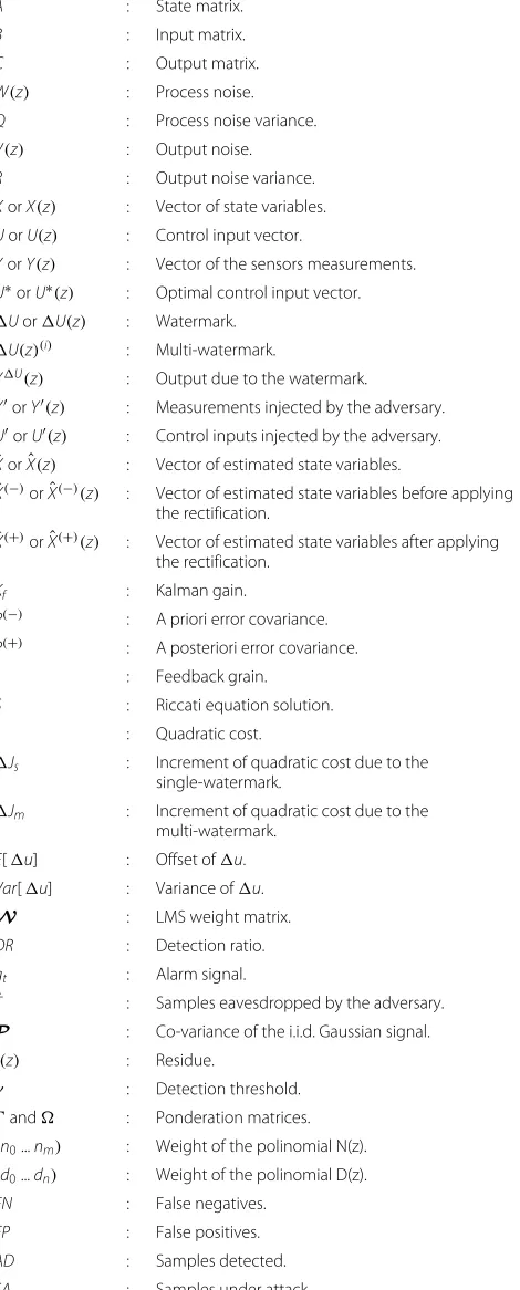
employed. In particular, this section is organized as fol-lows: in Section 3.1 we provide some necessary defini-tions and background concerning the class of control systems considered in this paper; Section 3.2 describes the attack detection scheme proposed in [4, 5]; in Section 3.3, we propose the cyber-physical adversaries; finally, in Section 3.4 we show methods that can be employed by the adversary to mislead the watermark-based detector. The notation used hereinafter is summarized in Table 1.

3.1 Definitions and background

We consider plants of industrial control systems that can be mathematically modeled as discrete linear time-invariant (LTI) systems. It is worth mentioning that a mathematical model provides a rigorous way to describe the dynamical behavior of a given system. In the follow-ing, we denote withX(z)theZ-transform of a signal xt, wheretis the time-discrete variable. Such class of systems can be described as follows:

zX(z)=AX(z)+BU(z)+W(z) (1)

whereX(z)is theZ-transform ofxt∈Rn, the vector of the state variables (or state) at the timestept,U(z)=Z{ut}is theZ-transform ofut ∈Rp, the control signal, andW(z) is theZ-transform ofwt ∈ Rn, the process noise that is assumed to be a white noise with zero mean and variance

Q, i.e.,wt ∼N(0,Q). Moreover,A∈Rn×nandB∈Rn×p are, respectively, thestatematrix and theinputmatrix.

A static relation maps the state X(z) to the system outputY(z), theZ-transform ofyt∈Rm:

Y(z) = CX(z)+V(z)

= C(zI−A)−1(BU(z)+W(z))+V(z) (2)

whereC ∈ Rm×n is the output matrix. The value of the output vectorY(z)represents the measurement produced by the sensors that is affected by a noiseV(z)that is theZ -transform ofvtassumed as a white noise with zero mean and varianceR, i.e.,vt∼N(0,R).

For the class of systems defined above, a widely used and effective control technique is the linear quadratic Gaussian (LQG) approach. The overall goal of an LQG controller is to produce a control law U(z) such that a quadratic costJ, that is function of both the statextand the control inputut, is minimized:

J= lim n→∞E

⎡ ⎣1

n n−1

j=0

xT_j xj+uTj uj ⎤

⎦ (3)

Table 1Notations used in this paper

A : State matrix.

B : Input matrix.

C : Output matrix.

W(z) : Process noise.

Q : Process noise variance.

V(z) : Output noise.

R : Output noise variance.

XorX(z) : Vector of state variables.

UorU(z) : Control input vector.

YorY(z) : Vector of the sensors measurements.

U∗orU∗(z) : Optimal control input vector. UorU₍z₎ : Watermark.

U(z)(i) _{: Multi-watermark.}

YU_{(z) : Output due to the watermark.}

YorY(z) : Measurements injected by the adversary.

UorU(z) : Control inputs injected by the adversary.

ˆ

XorXˆ(z) : Vector of estimated state variables.

ˆ

X(−)orXˆ(−)(z) : Vector of estimated state variables before applying the rectification.

ˆ

X(+)orXˆ(+)(z) : Vector of estimated state variables after applying the rectification.

Kf : Kalman gain.

P(−) : A priori error covariance. P(+) : A posteriori error covariance.

L : Feedback grain.

S : Riccati equation solution.

J : Quadratic cost.

Js : Increment of quadratic cost due to the single-watermark.

Jm : Increment of quadratic cost due to the multi-watermark.

E[u] : Offset ofu.

Var[u] : Variance ofu.

W : LMS weight matrix.

DR : Detection ratio.

gt : Alarm signal.

ˆ

T : Samples eavesdropped by the adversary.

P : Co-variance of the i.i.d. Gaussian signal.

r₍z₎ : Residue.

γ : Detection threshold.

and : Ponderation matrices. (n0...nm) : Weight of the polinomial N(z).

(d0...dn) : Weight of the polinomial D(z).

FN : False negatives.

FP : False positives.

AD : Samples detected.

SA : Samples under attack.

It is well-known that such a control problem has, under some unrestrictive technical conditions, an optimal solu-tion that, thanks to the separasolu-tion principle, is made of two components that can be designed independently:

1. a Kalman filter that, based on the noisy

measurements, produces an optimal state estimation ˆ

X(z)of the stateX(z);

2. a linear quadratic regulator (LQR) that, based on the state estimationXˆ(z), provides the control lawU(z) that solves the LQR problem (cf. Eq. (3)).

Let us briefly illustrate how these two components are designed. The Kalman filter estimates the state as follows:

• Predict (a priori) system stateXˆ(−)(z)and covariance:

ˆ

X(−)(z) = AXzˆ −1+BUz−1 P(−) = AP(+)z−1AT+Q • Update parameters and (a posteriori) system state

and covariance:

Kf =

P(−)CT CP(−)CT+R −1

ˆ

X(+) = ˆX(−)(z)+Kf

Y(z)−CXˆ(−)(z)

P(+) = I−KfC

P(−)

whereKf andP(+)denote, respectively, the Kalman gain and the a posteriori error covariance matrix, I is the identity matrix.

The optimal control lawU(z)provided by the LQR is a linear controller:

U(z)=LXˆ(+)(z) (4)

where Ldenotes the feedback gain of a linear-quadratic regulator (LQR) which minimizes the control cost (cf. Eq. 3) and it is defined as follows (cf. [4, 5] for further details):

L= −BTSB+−1BTSA,

withSbeing the matrix that solves the following discrete time algebraic Riccati equation:

S=ATSA+−ATSBBTSB+−1BTSA.

3.2 Theχ2detector

Before presenting the detection scheme, we provide a definition of the adversary model considered in [4, 5]:

Definition 3.1An attacker that has the ability to eaves-drop all the messages containing the sensor outputs Y(z) and to inject messages with an arbitrary signal Y(z) to conduct malicious actions is defined a cyber adversary.

Remark 3.2Notice that the definition given above does not suppose that the attacker possesses (or makes attempts to gather) any knowledge about the system model.

We denote withU∗(z)the output of the LQR controller given by Eq. (4) and with U(z) the control input that is sent to the plant (cf. Eq. (1)). The idea is to super-pose to the optimal control lawU∗(z)a watermark signal, U(z) = Z{ut},Z-transform ofut ∈ Rpthat serves as an authentication signal. Thus, the control inputU(z)

is given by

U(z)=U∗(z)+U(z) (5)

The watermark signal is a Gaussian random signal with zero mean that is independent both from the state noise

W(z)and the measurement noiseV(z). Such an authen-tication watermark is expected to detect replay and integrity attacks modeled by the adversary defined above. Now that the optimal control lawU∗(z)is equipped with the authentication signalU(z), a detector– physically co-located with the controller – can be designed having the goal of generating alarms when an attack takes place. Toward this end, [4, 5] propose to employ aχ2_{detector, a}

well-known category of real-time anomaly detectors clas-sically used for fault detection in control systems [20], for the purpose of attack detection.

Figure 2 shows the overall control system equipped with the attack detector proposed in [4, 5].

Fig. 2Overall control system equipped with the watermark-based detection scheme in [4, 5]

Analarm signal gtis computed based on the residues rt = Z−1{r(z)}, where r(z) = Y(z)− CXˆ(−) generated from the estimator. Then,gt is compared with a thresh-oldγ to decide whether the system is in a normal state. The threshold is tuned to minimize false alarms [4, 5]. The alarm signalgtis computed as follows:

gt= t

i=t−w+1

(ri)TP−1(ri) (6)

where w is the size of the detection window and P =

(CPCT+R)is the co-variance of an independent and iden-tically distributed (i.i.d.) Gaussian input signal from the sensors.

The system is considered not under attack if gt < γ, otherwise ifgt ≥γ the system is considered to be under attack and the detector generates an alarm.

3.3 Cyber-physical adversary

Let us assume the system employs the detector described in Section 3.2, so that the controller superposes its output with an authentication watermarkU(z). At steady-state, i.e., after the transient has been exhausted, the output of the system can be considered as the sum of its steady-state value and a component that is due to watermark signal that shall be only known by the controller.

Let us now introduce an enhanced adversary that is aware of the fact that the system employs theχ2

detec-tor presented above. Since the detecdetec-tor is based on a stationary watermark signal U(z), we will show that an adversary that is able to extract the model of the system from the control lawU(z)and the sensor measure-mentY(z) is able to conduct an attack while remaining undetected.

Definition 3.3An attacker that, in addition to the capa-bilities of the cyber adversary, is also able to eavesdrop the messages containing the output of the controller U(z)with the intention of improving its knowledge about the system model using a parametric or non-parametric identification model, is defined as a cyber-physical adversary.

Based on the way to model the system’s behavior, two different cyber-physical adversaries can be defined.

Definition 3.4An attacker that only uses the previous input and output of the system to identify the system model is defined as a non-parametric cyber-physical adversary.

to be, respectively, the output of the controller and the out-put of the measurement when an attack is taking place. We denote withu = Z−1{U}the watermark guessed by the non-parametric cyber-physical adversary.

Definition 3.6An attacker that is able to estimate the parameters of the system using input and output data to mislead the controller detector is defined as a parametric cyber-physical adversary.

Remark 3.7 A parametric cyber-physical adversary is able to estimate the parameters of the system using input and output data to mislead the controller detector. This adversary can use an ARX (autoregressive with exoge-nous input) model or an ARMAX (autoregressive-moving average with exogenous input) to estimate the model[22].

We assume that the main constraint of this adversary is the energy spent to eavesdrop and analyze the communi-cation data, i.e., the number of samples eavesdropped to obtain the system model parameters.

Proposition 3.8A cyber-physical adversary that is able to exactly estimate the system controlled by the controller cannot be detected by theχ2detector (cf.Eq. 6).

ProofWithout loss of generality, we assume an attack is started at timeT0, and we compute the residuesrtfor t∈[T0,T0+T−1]:

Z{rt} =Y(z)−CXˆ(−)z−(t−T0−1) (7) Moreover, it is easy to show that the following holds:

ˆ

X(−)z−(t−T0−1)=_Z ⎧ ⎨

⎩xˆt|t−T+At−T0

ˆ

xT0|T0−1− ˆxT0|T0−1

+ t−T0−1

i=0

Ai_Bu

t−1−i−ut−1−i ⎫⎬

⎭

= ˆX(−)z−(t−T−1)+

At−T0

×Xˆ(−)− ˆX(−)

z−(t−T0−1)

+ t−T0−1

i=0

Ai_B(U(z)

−U(z)z−(t−T0−1−i)

(8)

whereXˆis the estimated state when the system is under attack, andA=(A+BL)(I−KC)is a stable matrix [4, 5]. Substitution of (8) in (7) yields:

Z{rt} = Y(z)−CXˆ(−)

First term − C

At−T0 _Xˆ(−)− ˆ_X(−)

z−(t−T0−1)

Second term − C

t−T0−1 i=0

Ai_{B(U(z)−U(z))z}−(t−T0−1−i)

Third term

Let us consider separately the three terms in the equation written above: the first term follows the same distribution ofY(z)−CXˆ(−); sinceAis asymptotically stable — i.e., all its eigenvalues are inside the open unit disk of the complex plane — the second term converges exponentially fast to zero. In fact, the entries of At−T0 converge exponentially fast to zero. Now, if the third term is equal to zero, the dynamics of Z{rt} would recover the dynamics of the residues when no attack is under-going and thus, the attack would not be detected. Under the hypothesis of this proposition, the adversary knows exactly the watermark signal and thusU(z) = U(z)

which makes the third term equal to zero and concludes the proof.

3.4 Acquiring the watermark signal model

Motivated by Definition 3.4, we show now a practical method that can be used to acquire the watermark signal ut. In particular, we propose an adversary that employs a well known LMS (least mean square) adaptive FIR filter, a non-parametric identification model, with the purpose of running an online identification of the system model. With the identified model, it is possible to obtain the watermark and, finally, using it to authenticate messages with the aim of driving the system to an undesired state.

We denote withpthe LMS filter order and withμits step size. The step size μ is upper bounded by 2/λmax,

where λmax is the maximum eigenvalue of the

auto-correlation matrixR=E[XXH], whereXH is the Hermi-tian transpose, or conjugate transpose, ofX. Observe that ifμis chosen too small, the time to converge to optimal weights tends to be large [23]. The adversary initializes the

weight matrix W to be equal to the zero matrix. Then,

Algorithm 1 Non-parametric cyber-physical adversary algorithm

1: procedureADVERSARY ALGORITHM

2: k←length of eavesdropped data 3: p←filter order

4: j←p 5: top:

6: ifj<ktheni←1. 7: loop:

8: ifipthen

9: ini←j−p+1.

10: e(ini)←d(ini)−WTX[x(ini),. . .x(j)]. 11: W←W+μ¯e(ini)X[x(ini),. . .x(j)]. 12: j←j+i.

13: i←i+1. 14: go toloop.

15: close;

16: go totop.

Once the system model has been identified, the adver-sary is able to extract the watermark and carry out the replay attack. In particular, the adversary follows the steps described below:

1. Eavesdropping ofU(z)andY(z)and decomposition. The adversary captures both the control lawU(z)and the sensors outputY(z)to make the decomposition between the information data and the watermark using the LMS filter as a noise cancellation adaptive filter. With this first step, we are able to separate U∗(z)and the watermarkU(z)starting fromU(z). Notice that, since the system is linear, it follows from the superposition principle thatY(z)=Y∗(z)+YU, beingY∗(z)as the output due toU∗(z)andYU(z) as the output due to the watermarkU(z). 2. Acquiring the weight matrix,W. To acquire the

weight matrixW, the adversary uses the LMS adaptive filter described before; as a system identification method.

3. Computing the attack sensor measurementY(z). The adversary attacks the system by sending fake sensor measurementsY(z), whereYU(z)is computed using the watermarkU(z)as follows:

YU(z)=WTU(z)

andY(z)=Y∗(z)z−1+YU(z).

In the remainder of this section, we show via numeri-cal simulations that the detection mechanism proposed in [4, 5] is not sufficiently robust and is not able to detect cyber-physical adversaries (cf. Section 3.3) that are able to identify the system model by eavesdropping the data channel.

In order to simulate the scenario proposed in this section, we use a simplified version of the Tennesse East-man control challenge problem [24] (also used in [25]).

This system simulates a MIMO system of ordern = 7

withp= 4 inputs andm = 4 outputs. In particular, the model of the discrete LTI system described by Eqs. (1)–(2) is defined by the following matrices:

A= ⎡ ⎢ ⎢ ⎢ ⎢ ⎢ ⎢ ⎢ ⎢ ⎣

0.987 0 0 0 0 0 0

0 0.895 −0.025 0 0 0 0

0 0.036 0.999 0 0 0 0

0 0 0 1 −0.008 0 0

0 0 0 0.005 0.960 0 0

0 0 0 0 0 0.999 0

0 0 0 0 0 0 0.990

⎤ ⎥ ⎥ ⎥ ⎥ ⎥ ⎥ ⎥ ⎥ ⎦ , B= ⎡ ⎢ ⎢ ⎢ ⎢ ⎢ ⎢ ⎢ ⎢ ⎣

0.149 0 0 0

0 0 0 0.071

0 0 0 0.001

0.380 0 −0.096 0

1.000 0 −0.096 0

0 0.038 0 0

0 0 0 0.075

⎤ ⎥ ⎥ ⎥ ⎥ ⎥ ⎥ ⎥ ⎥ ⎦ , C= ⎡ ⎢ ⎢ ⎣

0.151 −0.076 0 0 0 0 0

0 0 0 0 1 0 0

0 0 0 0 0 0.040 0

0 0 0 0 0 0 0.133

⎤ ⎥ ⎥ ⎦.

Moreover, the co-variance matrices are equal toQ =

0.01IandR = I, whereas the cost matrices are = 1.5I

and=10I.

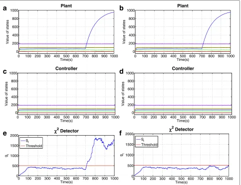
To validate our approach, we compare the system dynamics considering the two adversaries described above. Figure 3a, c shows the plant dynamics and the state estimated by the controller in the case of a cyber adversary. Figure 3a shows that the adversary is able to drive the state components to an undesired value. Never-theless, the controller, misled by the adversary, does not perceive such situation (cf. Fig. 3c). Figure 3b, d shows the dynamics of the plant and the ones of the controller under a non-parametric cyber-physical adversary model which exhibits the same behavior described above for the case of the cyber adversary.

0 100 200 300 400 500 600 700 800 900 1000 0

200 400 600 800 1000

Time(s)

Value of states

Plant

0 100 200 300 400 500 600 700 800 900 1000

0 200 400 600 800 1000

Time(s)

Value of states

Plant

0 100 200 300 400 500 600 700 800 900 1000

0 200 400 600 800 1000

Time(s)

Value of states

Controller

0 100 200 300 400 500 600 700 800 900 1000

0 200 400 600 800 1000

Time(s)

Value of states

Controller

0 100 200 300 400 500 600 700 800 900 1000

0 500 1000 1500 2000

Time(s) g t

χχχχ2

Detector

g t Threshold

0 100 200 300 400 500 600 700 800 900 1000

0 500 1000 1500 2000

Time(s) g t

χχχχ2

Detector

g t Threshold

a

b

c

d

e

f

Fig. 3Numeric simulation results. Attacks start att= 700 s.a,cThe dynamics of the state vector in the plant and in the controller under the cyber adversary attack.b,dThe dynamics of the state vector in the plant and in the controller under the non-parametric cyber-physical adversary attack. e,f_χ2_{detector results under the two aforementioned attack scenarios.aPlant states, cyber adversary attack.bPlant states, non-parametric}

cyber-physical adversary attack.cEstimated states in the controller, cyber adversary.dEstimated states in the controller, non-parametric cyber-physical adversary.eDetector results, cyber adversary.fDetector results, non-parametric cyber-physical adversary

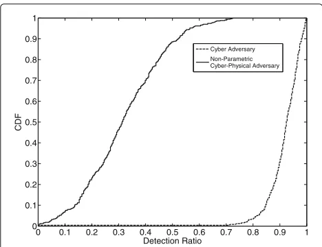
cyber-physical adversary (cf. Fig. 3f). Figure 3e shows that the detector is able to detect the cyber adversary thanks to the added watermark signal as soon as the attack starts att= 700 s. However, Fig. 3f shows that the same detector is not able to detect the non-parametric cyber-physical adversary sincegtdoes not exceed the threshold γ during the attack. In order to quantify the detector performance, we define a detection ratio (DR) metric as follows:

DR=

T₀+Ta

t=T0 1gt≥γ

Ta

(9)

where Ta is the attack duration, and 1 is the indica-tor function whose output is equal to 1 if the Boolean condition given as its argument (gt≥γ) is true; or 0

oth-erwise. In a nutshell, DR ∈[ 0, 1] can be considered as an efficiency index for the detector: DR is equal to 1 when the attack is always detected; and it is equal to 0 when the attack is always undetected.

0 0.1 0.2 0.3 0.4 0.5 0.6 0.7 0.8 0.9 1 0

0.1 0.2 0.3 0.4 0.5 0.6 0.7 0.8 0.9 1

Detection Ratio

CDF

Cyber Adversary Non-Parametric Cyber-Physical Adversary

Fig. 4Cumulative distribution function (CDF) of the detection ratio associated with theχ2detector (see Section 3.2), obtained by measuring the DR metric (see Eq. 9) for 200 simulations (both cyber and non-parametric cyber-physical adversary cases)

4 Multi-watermark-based attack detection In the previous section, we have defined three different kinds of adversaries who use different vulnerabilities of a control system to carry out attacks; cyber-adversary, non-parametric cyber-physical adversary, and parametric cyber-physical adversary. In this section, we propose a detection scheme that extends the one presented in [4, 5], in order to detect non-parametric cyber-physical adversaries. We also study the performance loss of the new detection scheme with regard to the one presented in [4, 5].

4.1 On the use of multi-watermark signals

The goal of our new detection scheme is to increase the difficulty in retrieving the authentication watermark U(z) from the control signal U(z), so that the prob-ability of detecting an attack from a non-parametric cyber-physical adversary can be increased. We assume that the control system under attack employs exactly the same type of controller and the same detection strat-egy presented in Section 3.2. The only difference in the proposed detection scheme is the way that the water-mark signalU(z)is generated. The control inputU(z), as in the case of the detection scheme presented in Section 3.2, is computed as the superposition of the optimal control signalU∗(z)produced by the LQR con-troller and a given multi-watermark signal U(z). The idea is to construct the authentication watermark

sig-nal by switching between N different and independent

processes with different co-variance and average (off-sets). More precisely, the non-stationary watermarkU

is obtained by periodically switching, with a period T,

betweenNsignalsU(i)_{, withi∈ I = {0, 1,. . .,N−1},} extracted by different stochastic processes. Hence,

the watermark signal U(z) can be formalized as

follows:

U(z)=Z

u(_ts(t,T))

(10)

wheres : N×R → I is a static function that maps the time samplet, and the switching periodT to an element of the index setIis defined as follows:

s(t,T)=

1

T mod (t,NT)

(11)

where mod(x,y)is the modulo operator, and ·is the floor function.

By using the proposed watermark (cf. Eq. 10), we now have an adaptive protection mechanism with two main configurable parameters: the number of distributions N

and the switching frequency f = 1/T. It is worth to notice that the original watermark signal described in

Section 3.2 is recovered whenf → 0 and whenU(0)

being a stationary zero mean Gaussian process.

4.2 Single-watermark LQG structure performance loss In this section, we compute the increment of cost in the LQG structure due to the single-watermark added to the control input. This supplementary cost is the degradation in the performance of the system, as shown in [5], and can be defined as follows:

J=J∗+Js (12)

where J∗ is the optimal cost of the system described in Section 3.1; andJs is the increment of cost due to the use of the single-watermark-based detector. In the fol-lowing, we develop the cost of the system in the time domain.

J = lim n→∞

1

n n−1

j=0 E

xT_j xj+uTj uj

= lim n→∞

1

n n−1

j=0

trCov(xj)+trCov(uj) (13)

wherextis defined as:

xt=Lx(wt,vt)+ ∞

j=t−1

andutas follows:

ut=Lu(wt,vt)+ ∞

j=t−1

(A+BL)jBVar(u−j)+V ar(ut)

(15)

whereLxandLuare linear functions. Their definition is not relevant for the target of this paper, but the reader can find the details in [5]. Assuming that the noise of the system and the watermark are independents, we can define the increment of cost due to the single-watermark as [5]:

Js=tr

⎡ ⎣Cov

⎛ ⎝∞

j=t−1

(A+BL)jBVar(u−j)

⎞ ⎠ ⎤ ⎦

−Ltr

⎡ ⎣Cov

⎛ ⎝∞

j=t−1

(A+BL)jBVar(u−j)+Var(ut)

⎞ ⎠ ⎤ ⎦

(16)

4.3 Multi-watermark LQG structure performance loss Let us now evaluate the increment of the cost gener-ated by the multi-watermark-based detector, Jm, and next, compare the cost generated by the single- and the multi-watermarks. The equation ofJm, is given by

Jm(t)=tr

⎡ ⎣Cov

⎛ ⎝∞

j=t−1

(A+BL)jBVaru₋(i)_j+Eu(₋i)_j

⎞ ⎠ ⎤ ⎦ +tr ⎡ ⎣LCov

⎛ ⎝∞

j=t−1

(A+BL)jB

Var(u(₋i)_j)+E

u(₋i)_j

+(Var(ut)+E[ut] ⎞ ⎠ ⎤ ⎦

(17)

where Var(u(_ti))andE[u(_ti)] are, respectively, the vari-ance and the mean of the watermark sent at moment

t. The performance loss of the LQG structure depends

linearly on the variance and the mean of the multi-watermarku(_ti)for eachTsamples.

The following theorem shows the difference between the performance loss due to the single-watermark, u, and the performance loss due to the multi-watermark, u(i).

Theorem 4.1Let us assume that a watermark is a Gaussian signal with a couple of parameters to be charac-terized; the mean and the variance. The multi-watermark

distribution is defined as Mw=N(E[u(i)] ,Var(u(i))), and the single-watermark distribution is defined as Sw = N(E[u] ,Var(u)). If we define for the multi-watermark βas:

β=E

u(i)

+Var

u(i)

∀i∈I (18)

and for the single-watermark as:

=E[u]+Var(u) (19)

where and β are constant for single- and multi-watermarks, respectively. Then, we can conclude that the performance loss of both approaches is equal if =β.

Proof If we assume that E[u]= 0 for the single-watermark, we can prove the theorem as follows:

Diff(Jm(t),Js(t))=Jm(t)−Js(t)

=tr

⎡ ⎣Cov

⎛ ⎝∞

j=t−1

(A+BL)jB(β₋j− −j) ⎞ ⎠ ⎤ ⎦

+Ltr

⎡ ⎣Cov

⎛ ⎝∞

j=t−1

(A+BL)jB(β₋j− −j)

+(βt− t) ⎞ ⎠ ⎤ ⎦₌0

Remark 4.2Note that using Theorem 4.1, the perfor-mance loss due to the multi and the single-watermark is equal. The assumption of the equal performance loss allows to compare both approaches under the same condi-tions. This can be formally stated as follows:

E

u(i)

+Var

u(i)

= =β. (20)

A= ⎡ ⎢ ⎢ ⎢ ⎢ ⎢ ⎢ ⎢ ⎢ ⎣

0.3991 0.07113 0.1573 −0.1274 0.0226 −0.0225 0.001

0.003 −0.07588 −0.005092 −0.03893 0.09917 −0.0168 0

−0.1974 −0.01849 0.0453 0.1579 −0.1597 0.1405 −0.002

−0.1246 −0.0726 0.1515 −0.1148 0.5156 −0.0665 0

0.4309 −0.1204 0.09715 0.055 0.2406 0.2812 0.0001

−0.0827 −0.01092 0.1234 −0.1318 0.0348 0.469 0

0.08312 −0.0829 0.081 0.0358 0.1124 0.02475 0.4469

⎤ ⎥ ⎥ ⎥ ⎥ ⎥ ⎥ ⎥ ⎥ ⎦ ,

B= ⎡ ⎢ ⎢ ⎢ ⎢ ⎢ ⎢ ⎢ ⎢ ⎣

0.947 0 0.002 −0.021

−0.0086 0 −0.406 0.02829

−0.8708 0.0011 0.0011 −0.106

0.4872 0.002 0.188 −0.041

0.1233 0 0.01 −0.9344

0 0 0 0.521

0 0.7658 0 0

⎤ ⎥ ⎥ ⎥ ⎥ ⎥ ⎥ ⎥ ⎥ ⎦ ,

C= ⎡ ⎢ ⎢ ⎣

−1.102 0.302 −0.1004 0.0386 0.053 0.0891 0

0 0.114 −0.0132 −1.087 0.116 0.051 0.905

0.0003 1.593 −0.002 0 0.093 0 0.0428

−0.163 −0.0712 −0.1074 0 0 −0.7443 0.089

⎤ ⎥ ⎥ ⎦.

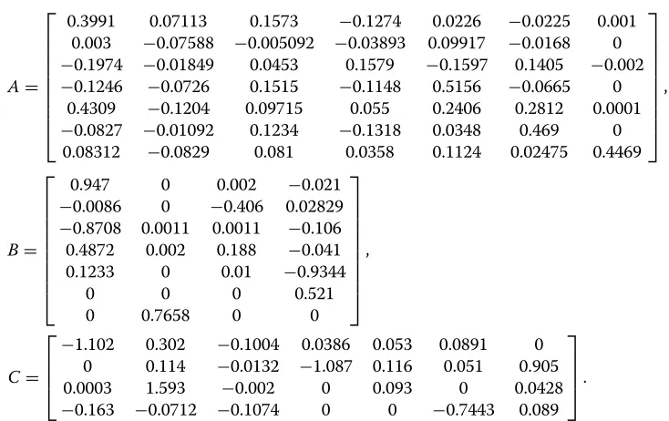
and co-variance matrices equal toQ = 0.2IandR = I. The positive definite cost matricesandare both equal to the identity matrix. The simulation is based on MAT-LAB and Simulink models of the plant, as well as the models of the non-parametric cyber-physical adversaries. The attacks start att= 700 s. We use three different dis-tributions (i.e.,N= 3) switched at random; a Gaussian, a Rician, and a Rayleigh distribution. Table 2 shows the co-variance and offset configured in the simulations for each distribution.

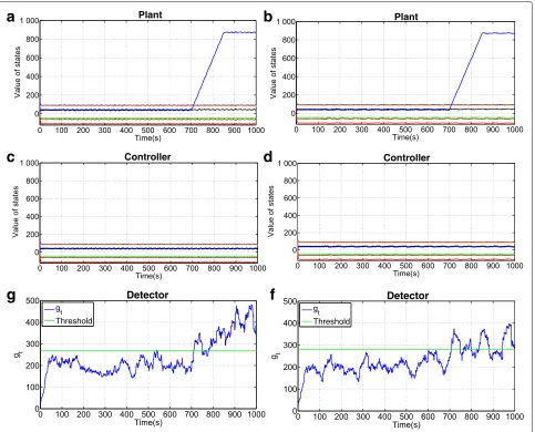
To validate the proposed attack–detection scheme, we compare the system dynamics considering two different switching frequencies. We have simulated a high fre-quency switching watermark configured to switch each 7 time samples, and a low frequency switching con-figured to switch each 20 time samples. Figure 5a, c shows the plant dynamics and the dynamics of the states estimated by the controller in the case of a switch-ing frequency watermark configured to 7 time sam-ples and a cyber-physical adversary attack. Figure 5a shows that the adversary is able to drive the state to an undesired value. Nevertheless, the controller misled by the adversary, does not perceive such situation (cf. Fig. 5c). Figure 5b, d shows the plant dynamics and

Table 2Sample parameters used in the multi-watermark MATLAB/Simulink implementation

Distribution Variance (_σ2_{) Offset}

Gaussian 5.9536 0.0

Rician 3.8870 3.7106

Rayleigh 3.0581 2.5553

the dynamics of the state estimated by the controller when the watermark is switched each 20 time samples. The dynamics show exactly the same behavior described above.

Figure 5e, f shows the dynamics of the alarm signalgt produced by the detector, respectively, in the case of high and low switching frequencies. Notice that switching the watermark distributions at a high frequency provides bet-ter detection performances compared to the case of a low switching frequency.

To quantify the effectiveness of the proposed detection scheme, we compute the detection ratio DR as a function of the switching frequency. In particular, for each con-sidered frequencyf we run 200 Monte Carlo simulations (with randomly generated system parameters) both in the case of the cyber-physical and the cyber adversary, and we compute the CDF (cumulative distribution function) of the detection ratio.

We start by confronting the performance obtained with the detection strategy based on multiple water-mark signals proposed in this paper with that pro-posed in [4, 5] in both the case of a cyber-physical and a cyber adversary. In the case of the proposed multi-watermark strategy, we consider two switching

fre-quencies fL = 0.05 Hz (switching watermark each 20

a

b

c

d

g

f

Fig. 5Numeric simulation results. Attacks start att= 700 s.a,bThe dynamics of the states vector in the plant under a non-parametric

cyber-physical adversary attack and switching frequency configured with two different configurations (0.14 and 0.05 Hz).c,dThe dynamics of the states vector estimated in the controller, under the same scenarios.e,fThe dynamics of the alarm signalgtproduced by the multi-watermark-based detector, under the same scenarios.aPlant states under a non-parametric cyber-physical adversary attack and switching frequency set to 0.14 Hz, i.e., every 7 timesteps, the controller changes the distribution associated with the watermark.bPlant states under a non-parametric cyber-physical adversary attack and switching frequency set to 0.05 Hz, i.e., every 20 timesteps, the controller changes the distribution associated with the watermark.cEstimated states in the controller under a non-parametric cyber-physical adversary attack and switching frequency set to 0.14 Hz.d Estimated states in the controller under a non-parametric cyber-physical adversary attack and switching frequency set to 0.05 Hz.eDetector results, switching frequency set to 0.14 Hz.fDetector results, switching frequency set to 0.05 Hz

particular, we notice that the detector employing a higher

switching frequency fH provides better performances

with respect to the case of using the lower switching frequencyfL.

In the following, we are interested in analyzing in more details the performance of the proposed detection strategy, when the switching frequency f is varied, to give a more in depth explanation of the anecdotal evi-dence shown above. Toward this end, Fig. 7a shows the CDF of the detection ratio obtained when the switch-ing frequency varies in the range 0.10–0.33 Hz. In

this case, we only consider cyber-physical adversaries. The CDFs shown in Fig. 7a confirm that when the switching frequency increases, the detection ratio also increases.

To finish this section, we provide in Fig. 7b the median detection ratio function off. The figure also contains the

case f = 0 that corresponds to the detection strategy

proposed in [4, 5] — used as a baseline. Theshaded area

0 0.1 0.2 0.3 0.4 0.5 0.6 0.7 0.8 0.9 1 0

0.2 0.4 0.6 0.8 1

Detection Ratio

CDF

(I) (II) (III) (IV)

Fig. 6Numeric simulation results using the single- and

multi-watermark detection schemes. Confronting the performance of the two detectors. (I)χ2detector in [4, 5] and cyber adversary. (II)χ2 detector and non-parametric cyber-physical adversary. (III) Multi-watermark detector with switching frequency set to 0.14 Hz and non-parametric cyber-physical adversary. (IV) Multi-watermark detector with switching frequency set to 0.05 Hz and non-parametric cyber-physical adversary

able to obtain a detection ratio that goes from around 0.2 in the case of the baseline approach of [4, 5] to around 0.6 in correspondence off = 0.33 Hz.

Observe that the probability of false alarms without attack (often referred in the related literature as false pos-itives) is fixed,α= 1%. Notice as well that false negatives

(i.e., undetected real attacks) are inversely proportional to the detection ratio for each switching frequency.

4.5 Efficiency validation

We have validated above the multi-watermark detector using a static function,I, to define the multi-watermark and different performance loss between single- and multi-watermarks. We next present the results and valida-tions obtained for a system with the same performance loss between single- and multi-watermark detectors and where the multi-watermark is generated from a non-static function, Id. Figure 8 shows the result obtained after running 200 Monte Carlo simulations of a system with single- and multi-watermark detectors against a non-parametric cyber-physical adversary. In this simulation, single- and multi-watermark detectors have 30% perfor-mance loss,J, with respect to the optimal cost. More-over, the watermark uses a dynamic function to define the multi-watermark. In Fig. 8a, we show the result of using both single- and multi-watermark for a system of order four. We can confirm that the multi-watermark detector, with the same performance loss as the single-watermark detector, has a higher detection ratio. Figure 8b shows the result of single- and multi-watermarks for a higher system of order, 25. On the one hand, these results confirm that the multi-watermark detector is able to detect properly non-parametric cyber-physical adversaries. Additionally, we can conclude that the detection ratio increases with the complexity of the system. On the other hand, Fig. 9 depicts that using the multi-watermark approach, with same performance loss as in the case of using only the

0 0.1 0.2 0.3 0.4 0.5 0.6 0.7 0.8 0.9 1

0 0.1 0.2 0.3 0.4 0.5 0.6 0.7 0.8 0.9 1

Detection Ratio

cdf

0.33Hz 0.25Hz 0.20Hz 0.16 Hz 0.14 Hz 0.12Hz 0.11Hz 0.10 Hz

a

b

Single_w f=0 Multi_w f=0.05 Multi_w f=0.14 Multi_w f=0.33 0

0.1 0.2 0.3 0.4 0.5 0.6 0.7 0.8 0.9 1

Detection Ratio

Watermark Based Detector f(Hz)

Single_w f=0 Multi_w f=0.05 Multi_w f=0.14 Multi_w f=0.33 0

0.1 0.2 0.3 0.4 0.5 0.6 0.7 0.8 0.9 1

Detection Ratio

Watermark Based Detector f(Hz)

a

b

Fig. 8Numeric simulation results using the single- and multi-watermark detection schemes with the same performance loss.aDetection ratio for a system of order four, using single- and multi-watermarks.bDetection ratio for a system of order 25, using single- and multi-watermarks.aDetection ratio function with respect to the single- and multi-watermarks with different switching frequencies for fourth order systems.bDetection ratio function with respect to the single- and multi-watermarks with different switching frequencies for systems of order 25

single-watermark, the detection ratio increases when the switching frequency varies in the range 0-0.14 Hz, where

f = 0 is the single-watermark detector. In the following section, we extend the analysis to the case of parametric cyber-physical adversaries.

4.6 Numerical validation of the multi-watermark detector against parametric cyber-physical adversaries In the previous sections, we have seen how the multi-watermark detector is able to detect both cyber and non-parametric cyber-physical adversaries. In this section, we

extend the study to the case of parametric cyber-physical adversaries (cf. Definition 3.6). We recall that paramet-ric cyber-physical adversaries are able to identify the system model parameters from the input and the out-put plant signals. In fact, a parametric cyber-physical adversary can obtain the system model with great accu-racy, if control commands and sensor measurements are accessible.

Let us first show how a parametric cyber-physical adversary acquires the watermark signal presented in [4, 5]. Remember that such a watermark is modeled as a

f=0 f=0.005 f=0.01 f=0.02 f=0.05 f=0.14 f=0.25 f=0.33 0

0.1 0.2 0.3 0.4 0.5 0.6 0.7 0.8 0.9 1

Detection Ratio

Watermark Based Detector f(Hz)

Gaussian signal with zero mean. Its variance is repre-sented byU, i.e.,ut ∼ N(0,U). The variance modifies the control inputs and propagates the modification to the system outputs. However, it does not modify the system dynamics. Control inputs are represented by

U(z)=U∗(z)+U(z) (21)

and the system outputs are represented by

Y(z) = H(z)(U(z)+W(z))+V(z)

= H(z)(U∗(z)+U(z)+W(z))+V(z) (22)

Using the aforementioned characteristic of the water-mark, a parametric cyber-physical adversary can use an ARX (autoregressive with exogenous input) model to define the system as follows [22]:

Y(z)=H(z)U(z)+V(z) (23)

whereU(z)andY(z)represent the inputs and the outputs of the plant, respectively; V(z) represents the external noise which affects the outputs of the plant; andH(z)is another way to describe the model of the system presented in Section 3, such that:

H(z)= N(z)

D(z) =

%

n0zm+n1zm−1+...+nm d0zn+d1zn−1+...+dn

& (24)

whereN(z)andD(z)are the polynomial functions which build the model of the system.

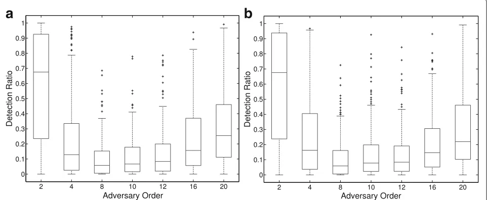
Following the same simulation setup introduced in Section 4.4, Figs. 10 and 11 show the detection ratio of the watermark detector against a parametric cyber-physical adversary. Figure 10 shows the results of 200 Monte Carlo simulations using systems of order 10 against this adversary. The results present the detec-tion ratio if the adversary uses a window size equal to 200 and different system orders for the model. If the adversary order varies in the range [8,12], the detec-tion ratio is not higher than 10%. Out of this range, the detection ratio increases drastically. Figure 11 shows the detection ratio using systems of order 25, against seven different parametric cyber-physical adversaries. The assumed window size is settled toTˆ = 300. The range of orders where the detection ratio does not increase drastically is [18, 28]. If an adversary uses an order in this range, the detection ratio is not higher than 10%. Otherwise, the likelihood to detect the adversary is high.

Figure 12 shows the detection ratio of the same sys-tem, against a parametric cyber-physical adversary with different window sizes (125, 150, 200, 250, and 300), and the correct system order. It is worth noting that the adversary needs a bigger window size in order to attack a system using a higher order, with a detection ratio less than 10%. Following the previous results, we can conclude that a parametric cyber-physical adversary, who is capable to eavesdrop and analyze a large num-ber of samples from the communication channel and use an equivalent order system, is capable of evading detection.

a

b

a

b

Fig. 11Numeric simulation results using the single- and multi-watermark detection schemes with the same performance loss, different adversary system order, and a window size equal to 300.aDetection ratio regarding single-watermark for systems of order 25.bDetection ratio regarding multi-watermark for systems of order 25.aDetection ratio function with respect to the single-watermark for systems of order 25 against a parametric cyber-physical adversary using different adversary system order.bDetection ratio function with respect to the multi-watermark for systems of order 25 against a parametric cyber-physical adversary using different adversary system order

Remark 4.3 A parametric cyber-physical adversary is able to obtain the system model, H(z), and mislead the con-troller, by eavesdropping the control inputs and the sensor measurements. The probability of being detected is equiv-alent to the probability of obtaining an erroneous model. This probability is directly proportional to the order of the system and inversely proportional to the window size to eavesdrop the data channel.

Following the Remark 4.3, and under the hypothesis of considering the real system like a black box, erroneous system identification depends on the order selected by the adversary to recreate the system model, as well as the number of eavesdropped samples and the window size used by the adversary to recompute the parame-ters of the target system. This situation can be quantified using mean squared error (MSE) [26, 27]. In a nutshell,

125 150 200 250 300

0 0.1 0.2 0.3 0.4 0.5 0.6 0.7 0.8 0.9 1

Detection Ratio

Adversary Windows Size

125 150 200 250 300

0 0.1 0.2 0.3 0.4 0.5 0.6 0.7 0.8 0.9 1

Detection Ratio

Adversary Window Size

a

b

the likelihood to obtain the correct model of the target system is directly proportional to the order chosen by the adversary to generate the model, and inversely pro-portional to the number of samples eavesdropped (cf. Figs. 10–12). The computational cost for the adversary is directly proportional to the system order, since the adver-sary needs to increase the order of the model, as well as the window size in order to minimize the MSE. Therefore, the number of samples eavesdropped before conduct-ing the attack, together with the order system chosen by the adversary, are the two main parameters to evade detection.

5 Experimental results with a laboratory SCADA testbed

In this section, we present some experimental results obtained with a real-world implementation of the detec-tion mechanisms and adversary models presented in this paper. The implementation is conducted using a labora-tory testbed based on SCADA protocols such as Modbus and DNP3 (cf. Section 2.1).

5.1 Testbed design

The architecture proposed for our SCADA testbed works as follows: all the elements (controller, sensors, actuators, PLCs, and RTUs) can be distributed across several nodes in a shared network combining DNP3 and Modbus pro-tocols (cf. Fig. 13). Likewise, one or various elements can be embedded into a single device. From a software standpoint, the controller never connects directly to the sensors. Instead, it is integrated in the architecture as a SCADA PLC node, with eventual connections to some other intermediary nodes. Such nodes are able to trans-late the controller commands into SCADA (e.g., either Modbus or DNP3) commands. As depicted in Fig. 13, the architecture is able to handle several industrial protocols and able to connect to complementary SCADA elements, such as additional PLCs and RTUs. To evolve the archi-tecture into a complete testbed, new elements can be included in the system, such as additional proxy-like RTU nodes.

From a data transmission standpoint, we include in our SCADA testbed the possibility of using differ-ent sampling frequencies, in order to cover a larger number of experimental scenarios. The architecture is able to handle several PLCs. To avoid overloading one channel with all the possible registers of the PLCs, separate ports are designated in order to isolate the communication between separated PLCs. DNP3 com-mands perform an Integrity Scan which gathers all the data from the PLCs in case several PLCs were being handled in the same channel, all variables of the a PLC would be fetched causing overhead in the communication.

5.2 Experimentation

We present in this section the results of applying the watermark authentication techniques proposed in this paper. Several repetitions of the experiments are orches-trated using automated scripts handling the elements of some representative scenarios. A set of attacks and detec-tors are used and posteriorly analyzed. The combinations, attack–detector, are the following:

• Replay attack–watermark disabled. In this scenario, the attacker is likely to evade the detector, since no watermark is injected into the system.

• Replay attack–watermark enabled. In this scenario, the attacker is likely identified by the detector, since the attack is not able to adapt to the current watermark.

• Non-parametric attack–stationary watermark. Using this scenario, the attacker and the detector have equal chances of success.

• Non-parametric attack–non-stationary watermark. Using this scenario, the non-stationary watermark changes the distribution systematically, hence, preventing the attack to adapt to such changes. The expected results are an increase of the detection ratio. • Parametric attack–stationary watermark. In this

scenario, the attacker is likely to evade the detector when the attack properly infers the system

parameters.

• Parametric attack–non-stationary watermark. The attacker is also likely to evade the detector when the system parameters are properly identified.

The cyber-physical implications of the testbed hinder the experimentation process especially when several rep-etitions are required in order to obtain statistical results, contrary to simulations where only the code is executed. The creation of the orchestration script, which automates the test, is necessary to simplify the experimentation tasks. The next section presents the results using the testbed for the aforementioned attacker-detector combi-nations. Some sample executions of the replay attack– watermark disabled scenario, as well as information about the implemented techniques, are available at http://j.mp/ TSPScada.

5.3 Experimention and results