DOI10.1186/2190-8567-2-2
R E S E A R C H Open Access
Gradient estimation in dendritic reinforcement learning
Mathieu Schiess·Robert Urbanczik·Walter Senn
Received: 12 May 2011 / Accepted: 15 February 2012 / Published online: 15 February 2012
© 2012 Schiess et al.; licensee Springer. This is an Open Access article distributed under the terms of the Creative Commons Attribution License (http://creativecommons.org/licenses/by/2.0), which permits unrestricted use, distribution, and reproduction in any medium, provided the original work is properly cited.
Abstract We study synaptic plasticity in a complex neuronal cell model where NMDA-spikes can arise in certain dendritic zones. In the context of reinforcement learning, two kinds of plasticity rules are derived, zone reinforcement (ZR) and cell reinforcement (CR), which both optimize the expected reward by stochastic gradient ascent. For ZR, the synaptic plasticity response to the external reward signal is mod-ulated exclusively by quantities which are local to the NMDA-spike initiation zone in which the synapse is situated. CR, in addition, uses nonlocal feedback from the soma of the cell, provided by mechanisms such as the backpropagating action poten-tial. Simulation results show that, compared to ZR, the use of nonlocal feedback in CR can drastically enhance learning performance. We suggest that the availability of nonlocal feedback for learning is a key advantage of complex neurons over networks of simple point neurons, which have previously been found to be largely equivalent with regard to computational capability.
Keywords Dendritic computation·reinforcement learning·spiking neuron
1 Introduction
Except for biologically detailed modeling studies, the overwhelming majority of works in mathematical neuroscience have treated neurons as point neurons, i.e., a linear aggregation of synaptic input followed by a nonlinearity in the generation of
M Schiess·R Urbanczik·W Senn (
)Department of Physiology, University of Bern, Bühlplatz 5, 3012 Bern, Switzerland e-mail:[email protected]
M Schiess
e-mail:[email protected]
R Urbanczik
somatic action potentials was assumed to characterize a neuron. This disregards the fact that many neurons in the brain have complex dendritic arborization where synap-tic inputs may be aggregated in highly nonlinear ways [1]. From an information pro-cessing perspective sticking with the minimal point neuron may nevertheless seem justified since networks of such simple neurons already display remarkable computa-tional properties: assuming infinite precision and noiseless arithmetic a suitable net-work of spiking point neurons can simulate a universal Turing machine and, further, impressive information processing capabilities persist when one makes more realis-tic assumptions such as taking noise into account (see [2] and the references therein). Such generic observations are underscored by the detailed compartmental model-ing of the computation performed in a hippocampal pyramidal cell [3]. There it was found that (in a rate coding framework) the input-output behavior of the complex cell is easily emulated by a simple two layer network of point neurons.
If the computations of complex cells are readily emulated by relatively simple cir-cuits of point neurons, the question arises why so many of the neurons in the brain are complex. Of course, the reason for this may be only loosely related to informa-tion processing proper, it might be that maintaining a complex cell is metabolically less costly than the maintenance of the equivalent network of point neurons. Here, we wish to explore a different hypothesis, namely that complex cells have crucial ad-vantages with regard to learning. This hypothesis is motivated by the fact that many artificial intelligence algorithms for neural networks assume that synaptic plasticity is modulated by information which arises far downstream of the synapse. A promi-nent example is the backpropagation algorithm where error information needs to be transported upstream via the transpose of the connectivity matrix. But in real axons any fast information flow is strictly downstream, and this is why algorithms such as backpropagation are widely regarded as a biologically unrealistic for networks of point neurons. When one considers complex cells, however, it seems far more plau-sible that synaptic plasticity could be modulated by events which arise relatively far downstream of the synapse. The backpropagating action potential, for instance, is of-ten capable of conveying information on somatic spiking to synapses which are quite distal in the dendritic tree [4,5]. If nonlinear processing occurred in the dendritic tree during the forward propagation, this means that somatic spiking can modulate synap-tic plassynap-ticity even when one or more layers of nonlinearities lie between the synapse and the soma. Thus, compared to networks of point neurons, more sophisticated plas-ticity rules could be biologically feasible in complex cells.
Fig. 1 Sketch of the neuronal cell model. Spatio-temporally clustered postsynaptic potentials (PSP,green) can give rise to NMDA-spikes (red) which superimpose additively in the soma (blue) controlling the generation of action potentials (AP).
an adequate minimal model of dendritic computation in basal dendritic structures, one should bear in mind that our model seems insufficient to describe the complex interactions of basal and apical dendritic inputs in cortical pyramidal cells [9,10].
2 Stochastic cell model of a neuron
We assume a neuron withN=40 initiation zones for NMDA-spikes, indexed byν=
1, . . . , N. An NMDA-zone is made up ofMν synapses, with synaptic strengthwi,ν
(i=1, . . . , Mν), where releases are triggered by presynaptic spikes. We denote by
Xi,νthe set of times when presynaptic spikes arrive at synapse(i, ν). In each
NMDA-zone, the synaptic releases give rise to a time varying local membrane potentialuν
which we assume to be given by a standard spike response equation
uν(t;X)=Urest+
Mν
i
wi,ν
s∈Xi,ν
(t−s). (1)
Here,Xdenotes the entire presynaptic input pattern of the neuron,Urest= −1 (ar-bitrary units) is the resting potential, and the postsynaptic response kernelis given by
ε(t )= (t ) τm−τs
(e−t /τm−e−t /τs).
We useτm=10 ms for the membrane time constant,τs=1.5 ms for the synaptic rise
time, andis the Heaviside step function.
The local potentialuν controls the rate at which what we call NMDA-events are
generated in the zone - in our model NMDA-events are closely related to the onset of NMDA-spikes as described in detail below. Formally, we assume that NMDA-events are generated by an inhomogeneous Poisson process with rate functionφN(uν(t;X)),
choosing
φN(x)=qNeβNx (2)
withqN=0.005 andβN=3. We adopt the symbolYν to denote the set of NMDA-event times in zoneν. For future use, we recall the standard result [19] that the prob-ability densityPw·,ν(Y
ν|X)of an event-trainYν generated during an observation
pe-riod running fromt=0 toT satisfies
logPw·,ν(Y
ν|X)=
T
0
dtlogqNeβNuν(t;X)
Yν(t )−q
NeβNuν(t;X), (3) whereYν(t )=s∈Yνδ(t−s)is theδ-function representation ofYν.
due to the second NMDA-event. Formally, we denote bysYν(t )=max{s≤t|s∈Yν}
the time of the last NMDA-event up to timet and model the somatic effect of an NMDA-spike by the response kernel
Yν(t )=
1 if 0≤t−sYν(t )≤=50 ms,
0 otherwise. (4)
The main motivation for modeling the generation of NMDA-spikes in this way is that it proves mathematically convenient in the calculations below. Having said this, it is worthwhile mentioning that treating NMDA-spikes as rectangular pulses seems reasonable, since their rise and fall times are typically short compared to the duration of the spike. Also, there is some evidence that increased excitatory presynaptic activ-ity extends the duration of a NMDA-spike but does not increase its amplitude [7,8]. Qualitatively, the above model is in line with such findings.
For specifying the somatic potentialUof the neuron, we denote byYthe vector of all NMDA-event trainsYν and byZthe set of times when the soma generates action potentials. We then use
U (t;Y, Z)=Urest+
N
ν=1
aYν(t )−
s∈Z
κ(t−s) (5)
for the time course of the somatic potential, where the reset kernelκ is given by
κ(t )=(t )e−t /τm.
This is a highly stylized model of the somatic potential since we assume that NMDA-zones contribute equally to the somatic potential (with a strength controlled by the positive parametera) and that, further, the AMPA-releases themselves do not con-tribute directly toU. Even if these restrictive assumptions may not be entirely un-reasonable (for instance, AMPA-releases can be much more strongly attenuated on their way to the soma than NMDA-spikes) we wish to point out that, while becoming simpler, the mathematical approach below does not rely on these restrictions.
Somatic firing is modeled as an escape noise process with an instantaneous rate functionφS(U (t;Y, Z))where
φS(x)=qSeβSx (6)
withqS=0.005 andβS=5. As shown in [20], for the probability densityP (Z|Y )of responding to the NMDA-events with a somatic spike trainZduring the observation period this implies
logP (Z|Y )=
T
0
dtlogqSeβSU (t;Z,Y)
Z(t )−qSeβSU (t;Z,Y) (7)
3 Reinforcement learning
In reinforcement learning, one assumes a scalar reward functionR(Z,X)providing feedback about the appropriateness of the somatic responseZto the inputX. The goal of learning is to adapt the synaptic strengths so as to obtain appropriate somatic re-sponses. For our neuronal model, the expected valueR¯of the reward signalR(Z,X)
is
¯ R(w)=
dXdYdZ P (X)Pw(Y|X)P (Z|Y)R(Z,X), (8)
whereP (X)is the probability density of the input spike patterns and Pw(Y|X)=
N
ν=1Pw·,ν(Y
ν|X). The goal of learning can now be formalized as finding aw
max-imizingR¯ and synaptic plasticity rules can be obtained using stochastic gradient as-cent procedures for this task.
In stochastic gradient ascent, X,Y, and Z are sampled at each trial and every weight is updated by
wi,ν←wi,ν+ηgi,ν(X,Y, Z),
where η >0 is the learning rate and gi,ν(X,Y, Z) is an (unbiased) estimator of ∂
∂wi,νR¯. Under mild regularity conditions, convergence to a local optimum is
guar-anteed if one uses an appropriate schedule for decreasingηtowards 0 during learning [21]. In biological modeling, one usually simply assumes a small but fixed learning rate.
The derivative ofR¯ with respect to the weight of synapse (i, ν)can be written as
∂ ∂wi,ν
¯
R=
dXdYdZ P (X)Pw(Y|X)P (Z|Y)R(Z,X)
∂ ∂wi,ν
logPw·,ν(Y
ν|X). (9)
Hence, a simple choice for the gradient estimator is
gi,νZR(X,Y, Z)=R(Z,X) ∂ ∂wi,ν
logPw·,ν(Y
ν|X) (10)
withPw·,ν(Y
ν|X)given by Equation3. Note that the conditional probabilityP (Z|Y)
does not explicitly appear in the estimator, so the update is oblivious of the architec-ture of the model neuron, i.e., of how NMDA-events contribute to somatic spiking. Since the only learning mechanism for coordinating the responses of the different NMDA-zones is the global reward signalR(Z,X), we refer to the update given by Equation10as ZR.
Better plasticity rules can be obtained by algebraic manipulations of Equations8
and9 which yield gradient estimators which have a reduced variance compared to Equation10- this should lead to faster learning. A simple and well-known example for this is adjusting the reinforcement baseline by choosing a constantcand replac-ingR(Z,X)withR(Z,X)+cin Equation 10; this amounts to addingc toR(w)¯
integrating outYin Equation8, yielding an estimator which directly considers the relationship between synaptic weights and somatic spiking because it is based on
∂
∂wi,νlogPw(Z|X). While actually doing the integration analytically seems
impracti-cal, we shall obtain estimators below from a partial realization of this program.
4 From zone reinforcement to cell reinforcement
Due to the algebraic symmetries of our model cell, it suffices to give explicit plasticity rules only for one synaptic weight. To reduce clutter we will thus focus on the first synapsew1,1in the first NMDA-zone.
4.1 Notational simplifications
LetY\denote the vector(Y2, . . . , YN)of all NMDA-event trains but the first andw\
the collection of synaptic weights(w.,2, . . . , w.,N)in all but the first NMDA-zone.
We rewrite the expected reward as
¯ R(w)=
dXdY\P (X)Pw\(Y\|X)r(w·,1,X,Y\) with
(11)
r(w·,1,X,Y\)=
dZdY1P (Z|Y)Pw·,1(Y
1|X)R(Z,
X).
Since in Equation11onlyrdepends onw1,1we just need to consider ∂w∂1,1r. Hence, we can regardXandY\as fixed and suppress them in the notation. This allows us to write the somatic potential (Equation5) simply as
U (t;Z, Y )=Ubase(t;Z)+aY(t ) (12)
using Y as shorthand for the NMDA-event trainY1 of the first zone and, further, incorporating into a time varying base potentialUbasethe following contributions in Equation5: (i) the resting potential, (ii) the influence ofY\, i.e., NMDA-events in the other zones, (iii) any reset caused by somatic spiking. Similarly, the notation for the local membrane potential of the first NMDA-zone becomes
u(t )=ubase(t )+wψ (t ), (13)
wherewstands for the strengthw1,1 of the first synapse,ψ (t )=
s∈X1,1(t−s),
and the effect of the other synapses impinging on the zone is absorbed intoubase(t ). Finally, thew-dependent contributionrto the expected reward (Equation11) can be written as
r(w)=
dZdY P (Z|Y )Pw(Y )R(Z), (14)
where also forR andPw we have suppressed the dependence onX. In the reduced
estimator in ZR-learning is
gZR(Y, Z)=R(Z)
T
0
dtY(t )−qNeβNu(t )
βNψ (t ). (15)
4.2 Cell reinforcement
To simplify the manipulation of Equation14, we replace the Poisson process generat-ingY by a discrete time process with step-sizeδ >0. We assume that NMDA-events inY can only occur at timestk=kδwherekruns from 1 toK= T /δand
intro-duceKindependent binary random variablesyk∈ {0,1}to record whether or not a
NMDA-event occurred. For the probability of not having a NMDA-event at timetk
we use
Pw(yk=0)=e−δφN(u(tk)). (16)
With this definition, we can recover the original Poisson process by taking the limit
δ→ +0. We usey=(y1, . . . , yK)to denote the entire response of the NMDA-zone
and, to make contact with the set-based description of the NMDA-trains, we denote byyˆ the set of NMDA-event times iny, i.e.,yˆ= {tk|yk=1}. Next, the discrete time
version of Equation14is
rδ(w)=
dZ
y
R(Z)P (Z|ˆy)Pw(y), (17)
wherePw(y)=
K
k=1Pw(yk). In the end, we will recoverr fromrδ by takingδ to
zero.
The derivative of Equation17is
∂ ∂wrδ=
dZ
y
P (Z|ˆy)Pw(y)R(Z) K
k=1
∂
∂wlogPw(yk)
and to focus on the contributions to ∂w∂ rδfrom each time bin we set
gradk=
dZ
y
Pw(y)P (Z|ˆy)R(Z)
∂
∂wlogPw(yk). (18)
Hence,∂w∂ rδ=
K
k=1gradk.
We now exploit the trivial fact that we can think ofP (Z|ˆy)as a function linear in
yk, simply becauseyk is binary. As a consequence, we can decomposeP (Z|ˆy)into
two terms: one which depends onyk and one which does not. For this, we pick a
scalarμand rewriteP (Z|ˆy)as
wherey\k=(y1, . . . , yk−1, yk+1, . . . , yK)and
α(y\k)=μP (Z|ˆy∪ {tk})+(1−μ)P (Z|ˆy\ {tk})
β(y\k)=P (Z|ˆy∪ {tk})−P (Z|ˆy\ {tk}).
Plugging Equation19into Equation18yields gradk as sum of two terms
gradk=Ak+Bk where
Ak=
dZ
y
Pw(y)α(y\k)R(Z)
∂
∂wlogPw(yk) (20)
Bk=
dZ
y
Pw(y)R(Z)(yk−μ)β(y\k)
∂
∂wlogPw(yk).
Rearranging terms inAk, we get
Ak=
dZ
y\k
Pw(y\k)R(Z)α(y\k)
yk
Pw(yk)
∂
∂wlogPw(yk).
Now,y
kPw(yk)
∂
∂wlogPw(yk)=
yk
∂
∂wPw(yk)= ∂
∂w1=0, hence
Ak=0 and gradk=Bk. (21)
The two equations above encapsulate our main idea for improving on ZR. In show-ing thatAk=0 we summed over the two outcomes yk∈ {0,1}, thus identifying a
noise contribution in the ZR estimatorR(Z)∂w∂ logPw(yk)for gradkwhich vanishes
through the averaging by the sampling procedure. Note that the remaining contribu-tionBk has as factorβ(y\k), a term which explicitly reflects how a NMDA-event at
timetkcontributes to the generation of somatic action potentials. In going from
Equa-tion20to Equation21, we assumed that the parameterμwas constant. However, a quick perusal of the above derivation shows that this is not really necessary. For jus-tifying Equation21, one just needs thatμdoes not depend onyk, so thatα(y\k)is
indeed independent ofyk. In the sequel, it shall turn to be useful to introduce a value
ofμwhich depends on somatic quantities.
A drawback of Equations20and21is that they do not immediately lend them-selves to Monte-Carlo estimation by sampling the process generating neuronal events. The reason being the missing termP (Z| ˆy) in the formula forBk. To
rein-troduce the term, we set
˜
βy(tk)=β(y\k)/P (Z|y) (22)
and in view of Equations20and21have
gradk=
dZ
y
Pw(y)P (Z|y)R(Z)(yk−μ)β˜y(tk)
∂
Hence, R(Z)(yk −μ)β˜y(tk)∂w∂ logPw(yk) is an unbiased estimator of gradk and,
since gradkgives the contribution to ∂w∂ rδfrom thekth time step,
gδCR=R(Z)
K
k=1
(yk−μ)β˜y(tk)
∂
∂wlogPw(yk) (23)
is an unbiased estimator of ∂w∂ rδ. Note that, while unavoidable, the above recasting
of the gradient calculation as an estimation procedure does seem risky. Due to the division byP (Z|y)in introducingβ˜, Equation22, rare somatic spike trainsZ can potentially lead to large values of the estimatorgCRδ .
To obtain a CR estimatorgCRfor the expected rewardR¯in our original problem, we now just need to takeδ to 0 in Equation 23and tidy up a little. The detailed calculations are presented in Appendix1, here we just display the final result:
gCR(Y, Z)=R(Z)
T
0
dt(1−μ)(1−e−γY(t ))Y(t )
+μ(eγY(t )−1)q
NeβNu(t )
βNψ (t ),
γY(t )=log
P (Z|Y ∪ {t})
P (Z|Y\ {t}) (24)
=
min(T ,t+) t
ds1−Y\{t}(s)
×aβSZ(s)−qS(eaβS−1)eβSUbase(s;Z)
.
In contrast to the ZR-estimator,gCRdepends on somatic quantities viaγY(t )which assesses the effect of having a NMDA-event at timet on the probability of the ob-served somatic spike train. This requires the integration over the duration of a NMDA-spike.
The CR-rule can be written as the sum of two terms, a time-discrete one depending on the NMDA-eventsY, and a time-continuous one depending on the instantaneous NMDA-rate, both weighted by the effect of an NMDA-event on the probability of producing the somatic spike train:
gCR(Y, Z)=(1−μ)R(Z)
T
0
dt P (Z|Y ∪ {t})−P (Z|Y\ {t})
P (Z|Y∪ {t}) Y(t )βNψ (t )
+μR(Z)
T
0
dtP (Z|Y∪ {t})−P (Z|Y\ {t}) P (Z|Y\ {t}) qNe
βNu(t )β
Nψ (t ).
5 Performance of zone and cell reinforcements
incorrect response, resulting in rewardR(Z,X)= −1. The correct response is not to spike (Z= ∅) and this results in a reward of 0. With these reward signals, synaptic updates become less frequent as performance improves. This compensates somewhat for having a constant learning rate instead of the decreasing schedule which would ensure proper convergence of the stochastic gradient procedure. We usea=0.5 for the NMDA-spike strength in Equation5, so that just 2-3 concurrent NMDA-spikes are likely to generate a somatic action potential. The input patternXis held fixed and initial weight values are chosen so that correct and incorrect responses are equally likely before learning. Simulation details are given in Appendix2. Given our choice ofaand the initial weights, dendritic activity is already fairly low before learning and decreasing it to a very low level is all that is required for good performance in this simple task (Figure2).
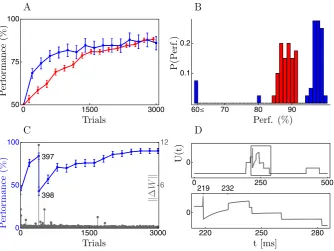
Simulations for ZR and CR (with a constant value of μ= 12) are shown in panel 6A. Given the sophistication of the rule, the performance of CR is disappoint-ing, yielding on average only a modest improvement over ZR. The histogram in panel 6B shows that in most cases CR does in fact learn substantially faster than ZR but, in contrast to ZR, CR spectacularly fails on some runs. Performance in a bad run of the CR-rule is shown in panel 6C, revealing that performance can deteriorate in a single trial. In this trial, a very unlikely somatic response was observed (panel 6D), resulting in a large value ofγY, thus leading to an excessively large change in synaptic strength.
The finding that large fluctuations in the CR-estimator can arise from rare somatic events, confirms the suspicion in Section4.2that recasting Equation20as a sampling procedure can lead to problems. Luckily, this can be addressed using the additional degree of freedom provided by the parameterμin the CR-rule. To dampen the effect of the fluctuations inγY, we setμto the time-dependent value
μ= 1
1+eγY(t )=
P (Z|Y\ {t})
P (Z|Y ∪ {t})+P (Z|Y\ {t}). (25)
Note thatμ is independent of whether or nott ∈Y. Hence, in view of our remark following Equation21, this is in fact a valid choice forμ. The specific form of Equa-tion25is to some extent motivated by the aesthetic considerations. It simplifies the first line of Equation24to
gbCR(Y, Z)=R(Z)
T
0
dt tanh 1
2γY(t ) Y(t )+qNe
βNu(t )β
Nψ (t ). (26) We refer to this estimator as balanced cell reinforcement (bCR) (Figure3).
From the third line of Equation24, one sees that the somato-dendritic interaction term in Equation26 can be written as tanh(12γY(t ))= P (ZP (Z||YY∪{∪{tt}}))−+P (ZP (Z||YY\{\{tt}})). This highlights the terms role as assessing the relevance to the produced somatic spike train of having an NMDA-event at timet. In this, it is analogous to thee±γYterms in
Fig. 2 Learning to stay quiescent.(A)Learning curves for cell reinforcement (blue) and zone reinforce-ment (red) when the neuron should not respond with any somatic firing to one pattern which is repeatedly presented. Values shown are averages over 40 runs with different initial weights and a different input pattern.(B)Distributions of the performance after 1500 trials.(C)A bad run of the CR-rule where per-formance drops dramatically after the 397th pattern presentation. The grey points show the Euclidean norm of the changeWin the neurons weight matrixW, highlighting the excessively large synap-tic update after trial 397.(D)Time course of the somatic potential during trial 397 (the straight line att=219 ms marks a somatic spike). As shown more clearly by the blow-up in the bottom row an NMDA-spike occurring att∗=232 ms yields a value ofUwhich stays strongly positive for some 10 ms. (Udrops thereafter because a NMDA-spike in a different zone ends.) Improbably, however, the sustained elevated value ofU aftert∗does not lead to a somatic spike. Hence, the likelihood of the observed so-matic responseZgiven the activityYνin the zoneνwhere the NMDA-spike at timet∗occurred is quite small,P (Z[t∗,t∗+]|Yν)=P (Z[t∗,t∗+]|Yν∪ {t∗})≈0.017. Indeed, the actual somatic response would have been much more likely without the NMDA-spike,P (Z[ts,ts+]|Yν\ {t∗})≈0.72. The discrepancy
between the two probabilities yields a large value of exp(−γYν(t∗))in Equation24, leading to the strong weight change. Error bars in the figure show 1 SEM.
the expected rate. In bCR, this difference has become a sum. Hence, exploration at the NMDA-event level is only of minor importance for the bCR-rule, where the essential driving force for plasticity is the somatic exploration entering through the factor tanh(12γY).
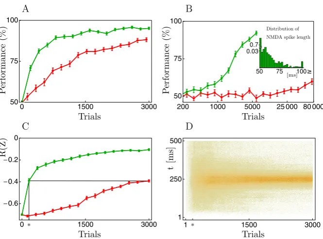
Fig. 3 Balanced cell reinforcement (bCR, Equation26) compared to zone reinforcement.(A)Average performance of bCR (green) and ZR (red) on the same task as in panel 6A.(B)Performance when learning stimulus-response associations for four different patterns; bCR (green), ZR (red), a logarithmic scale is used for thex-axis. The inset shows the distribution of NMDA-spike durations after learning the task with bCR. The performance values in the figure are averages over 40 runs, and error bars show 1 SEM.
(C)Development of the average reward signalR(Z)for bCR (green) and ZR (red) when the task is to spike at the mid time of the single input pattern (R(Z)= −2/(nT )i|tisp−ttarg|, wheretisp∈Z,i=1, . . . , n, is theith of thenoutput spike times,ttarg=250 ms the target spike time, andT =500 ms the pattern duration; if there was no output spike within[0, T )we added one atT, yieldingR(Z)= −1).(D)Spike raster plot of the output spike timesZwithR(Z)shown in C using bCR. With ZR, the distribution of spike times after 3000 trials roughly corresponds to the one for bCR after 160 trials (vertical line at∗), where the two performances coincide (see∗andblack linesin C). The mean and standard deviation of the spike times at the end of the learning process, averaged across the last 300 trials, was 251±45 and 256±121 ms for bCR and ZR, respectively.
the other two patterns the correct response was to stay quiescent. One of the four stimulus-response associations was randomly chosen on each trial and, as before, cor-rect somatic responses lead to a reward signal ofR=0 whereas incorrect responses resulted inR= −1. The inset to panel 5B shows the distribution of NMDA-spike du-rations after learning the four stimulus-response associations with bCR. Over 70% of the NMDA-spikes last for just a little longer than the minimal length of=50 ms. Further nearly all of the spikes are shorter than 100 ms, thus staying well within a physiologically reasonable range.
6 Discussion
We have derived a class of synaptic plasticity rules for reinforcement learning in a complex neuronal cell model with NMDA-mediated dendritic nonlinearities. The novel feature of the rules is that the plasticity response to the external reward signal is shaped by the interaction of global somatic quantities with variables local to the dendritic zone where the nonlinear response to the synaptic release arises. Simulation results show that such so-called CR rules can strongly enhance learning performance compared to the case where the plasticity response is determined just from quantities local to the dendritic zone.
In the simulations, we have considered only a very simple task with a single complex cell learning stimulus-response associations. The results, however, show that compared to ZR the bCR rule provides a less noisy procedure for estimating the gradient of the log-likelihood of the somatic response given the neuronal input (∂w∂
i,νlogPw(Z|X)). Estimating this gradient for each neuron is also the key step for
reinforcement learning in networks of complex cells [13]. Further, simply memoriz-ing the gradient estimator with an eligibility trace until reward information becomes available, yields a learning procedure for partially observable Markov decision pro-cesses, i.e., tasks where the somatic response may have an influence on which stim-uli are subsequently encountered and where reward delivery may be contingent on producing a sequence of appropriate somatic responses [22–24]. The quality of the gradient estimator is a crucial factor also in these cases. Hence, it is safe to assume that the observed performance advantage of the bCR rules carries over to learning scenarios which are much more complex than the ones considered here.
In this investigation, we have adopted a normative perspective, asking how the different variables arising in a complex neuronal model should interact in shaping the plasticity response - striving for maximal mathematical transparency and not for maximal biological realism. Ultimately, of course, we have to face the question of how instructive the obtained results are for modeling biological reality. The question has two aspects which we will address in turn: (A) Can the quantities shaping the plasticity response be read-out at the synapse? (B) Is the computational structure of the rules feasible?
(A) The global quantities in CR are the timing of somatic spikes as well as the value of the somatic potential. The fact that somatic spiking can modulate plasticity is well established by STDP experiments (spike timing-dependent plasticity). In fact such experiments can also provide phenomenological evidence for the modulation of synaptic plasticity by the somatic potential, or at least by a low-pass filtered version thereof. The evidence arises from the fact that the synaptic change for multiple spike interactions is not a linear superposition of the plasticity found when pairing a single pre-synaptic and a somatic spike. Explaining the discrepancy seems to require the introduction of the somatic potential as an additional modulating factor [25].
In CR-learning, however, we assume that the somatic potentialU (Equation5) can differ substantially from a local membrane potentialuν (Equation1) and both
current flow into the neuron and the flow resulting from AMPA-releases in its local dendritic NMDA-zone. While the differential contribution of the two flows is going to be indistinguishable in any local potential reading, the difference could conceivably be established from the detailed ionic composition giving rise to the local potential at the synapse. A second, perhaps more likely, option arises when one considers that spiking is widely believed to rely on the pre-binding of Glutamate to NMDA-receptors [7]. Hence,uν could simply be the level of such NMDA-receptor bound
Glutamate, whereasU is relatively reliably inferred from the local potential. Such a reinterpretation does not change the basic structure of our model, although it might require adjusting some of the time constants governing the build up ofuν.
(B) The plasticity rules considered here integrate over the durationT correspond-ing to the period durcorrespond-ing which somatic activity determines eventual reward delivery. But synapses are unlikely to know when such a period starts and ends. As in pre-vious works [12,18], this can be addressed by replacing the integral by a low-pass filter with a time constant matched to the value ofT. The CR-rules, however, when evaluatingγY(t )to assess the effect of an NMDA-spike, require a second integration extending from timet into the future up tot+. The acausality of integrating into the future can be taken care of by time shifting the integration variable in the first line of Equation24, and similarly for Equation26. But the time shifted rules would require each synapse to buffer an impressive number of quantities. Hence, further ap-proximations seem unavoidable and, in this regard, the bCR-rule (Equation26) seem particularly promising due to its relatively simple structure. Approximating the hy-perbolic tangent in the rule by a linear function yields an update which can be written as a proper double integral. This is an important step in obtaining a rule which can be implemented by a biologically reasonable cascade of low-pass filters.
Appendix 1
Here, we detail the steps leading from Equation22forgδCRto Equation24forgCR. We first obtain a more explicit form forgδCR. In view of Equation22,β˜y(tk)= P (Z|ˆy∪{tk})
P (Z|ˆy/{tk}) −1 if yk =0, whereas β˜y(tk)=1−
P (Z|ˆy/{tk})
P (Z|ˆy∪{tk}) if there is
NMDA-triggering at timetk. Hence, setting
γY(t )=log
P (Z|Y∪ {t})
P (Z|Y \ {t}) we have β˜y(tk)=(2yk−1)
1−eγyˆ(tk)(1−2yk)
and hence
gCRδ (Y, Z)=R(Z)
K
k=1
(yk−μ)(2yk−1)
1−eγyˆ(tk)(1−2yk ) ∂
∂wlogPw(yk).
Further, from Equation16,
∂
∂wlogPw(yk=1)=βNψ (tk)+O(δ), ∂
∂wlogPw(yk=0)= −δβNqNe
βNu(tk)ψ (t
k).
Hence, taking the limitδ→0, we obtain
gCR(Y, Z)=R(Z)
T
0
dt βNψ (t )
(1−μ)(1−e−γY(t ))Y(t )
−qNeβNu(t )μ(1−eγY(t ))
,
equivalent to the first equation in Equation24.
We next need an explicit expression forγY(t ). Going back to its definition (Equa-tion24) and using Equations7and12yields
γY(t )= T
0
log(qSeβSU (s;Z,Y∪{t}))Z(s)−qSeβSU (s;Z,Y∪{t}) ds − T 0
log(qSeβSU (s;Z,Y\{t}))Z(s)−qSeβSU (s;Z,Y\{t})
ds
=
T
0
βS(U (s;Z, Y ∪ {t})−U (s;Z, Y\ {t}))Z(s)ds
−
T
0
qS
eβSU (s;Z,Y∪{t})−eβSU (s;Z,Y\{t})ds
=
T
0
βSa
Y∪{t}(s)−Y\{t}(s)
Z(s)ds
−
T
0
qSeβSUbase(s;Z)
We next note that timessoutside of the interval [t, t+]do not contribute to the above integrals sinceY∪{t}(s)=Y\{t}(s)for such s. Further, Y∪{t}(s)=1 for
s∈ [t, t+]. Hence,
γY(t )=
min(T ,t+) t
ds aβS
1−Y\{t}(s)
Z(s)
−qSeβSUbase(s;Z)
eaβS−eaβSY\{t}(s).
For the term in square brackets we note that, sinceY\{t}(s)is zero or one,eaβS−
eaβSY\{t}(s)=eaβS −(1−
Y\{t}(s)+eaβSY\{t}(s))=(eaβS−1)(1−Y\{t}(s)).
Hence, finally,
γY(t )=
min(T ,t+) t
ds1−Y\{t}(s) aβSZ(s)−qS(eaβS−1)eβSUbase(s;Z)
which gives the last line of (Equation24).
Appendix 2
Here, we provide the remaining simulation details.
An input pattern has a duration ofT =500 ms and is made up from 150 fixed spike trains chosen independently from a Poisson process with a mean firing rate of 6 Hz (independent realizations are used for each pattern). We think of the input as being generated by an input layer with 150 sites, with each NMDA-zone having a 50% probability of being connected to one of the sites. Hence, on average a NMDA-zone receives 75 input spike trains and 37.5 spike trains are shared between any two NMDA-zones.
A roughly optimized learning rate was used for all tasks and learning rules. Roughly, optimized means that the used learning rateη∗yields a performance which is better that when using 1.5η∗orη∗/1.5.
In obtaining the learning curves, for each run a moving average of the actual trial by trial performance was computed using an exponential filter with time constant 0.1. Mean learning curves where subsequently obtained by averaging over 40 runs. The exception to this is the single run learning curve in panel 6C. There, subsequently to each learning trial, 100 non-learning trials were used for estimating mean perfor-mance.
Initial weights for each run were picked independently from a Gaussian with mean and variance equal to 0.5. Euler’s method with a time step of 0.2 ms was used for numerically integrating the differential equations.
Competing interests
Acknowledgements This study was supported by the Swiss National Science Foundation (SNSF, siner-gia grant CRSIKO 122697/1) and a grant of the Swiss SystemsX.ch initiative (Neurochoice, evaluated by the SNSF).
References
1. Polsky A, Mel BW, Schiller J:Computational subunits in thin dendrites of pyramidal cells.Nat NeurosciJun 2004,7:621-627.
2. Maass W:Computation with spiking neurons. InThe Handbook of Brain Theory and Neural Net-works. Edited by Arbib MA. Cambridge: MIT Press; 2003:1080-1083.
3. Poirazi P, Brannon T, Mel BW:Pyramidal neuron as two-layer neural network.NeuronMar 2003,
37:989-999.
4. Nevian T, Larkum ME, Polsky A, Schiller J:Properties of basal dendrites of layer 5 pyramidal neurons: a direct patch-clamp recording study.Nat NeurosciFeb 2007,10:206-214.
5. Zhou WL, Yan P, Wuskell JP, Loew LM, Antic SD:Dynamics of action potential backpropagation in basal dendrites of prefrontal cortical pyramidal neurons.Eur J NeurosciFeb 2008,27 :923-936.
6. Schiller J, Major G, Koester HJ, Schiller Y:NMDA spikes in basal dendrites of cortical pyramidal neurons.NatureMar 2000,404:285-289.
7. Schiller J, Schiller Y:NMDA receptor-mediated dendritic spikes and coincident signal amplifi-cation.Curr Opin NeurobiolJun 2001,11:343-348.
8. Major G, Polsky A, Denk W, Schiller J, Tank DW:Spatiotemporally graded NMDA spike/plateau potentials in basal dendrites of neocortical pyramidal neurons. J Neurophysiol May 2008,
99:2584-2601.
9. Larkum ME, Zhu JJ, Sakmann B:A new cellular mechanism for coupling inputs arriving at dif-ferent cortical layers.NatureMar 1999,398:338-341.
10. Larkum ME, Nevian T, Sandler M, Polsky A, Schiller J:Synaptic integration in tuft dendrites of layer 5 pyramidal neurons: a new unifying principle.ScienceAug 2009,325:756-760.
11. Seung H:Learning in spiking neural networks by reinforcement of stochastic synaptic transmis-sion.Neuron2003,40:1063-1073.
12. Fremaux N, Sprekeler H, Gerstner W:Functional requirements for reward-modulated spike-timing-dependent plasticity.J NeurosciOct 2010,30:13326-13337.
13. Williams R:Simple statistical gradient-following algorithms for connectionist reinforcement learning.Mach Learn1992,8:229-256.
14. Matsuda Y, Marzo A, Otani S:The presence of background dopamine signal converts long-term synaptic depression to potentiation in rat prefrontal cortex.J Neurosci2006,26:4803-4810. 15. Seol G, Ziburkus J, Huang S, Song L, Kim I, Takamiya K, Huganir R, Lee H, Kirkwood A:
Neu-romodulators control the polarity of spike-timing-dependent synaptic plasticity.Neuron2007,
55:919-929. Erratum in:Neuron56:754.
16. Pawlak V, Kerr JN:Dopamine receptor activation is required for corticostriatal spike-timing-dependent plasticity.J NeurosciMar 2008,28:2435-2446.
17. Werfel J, Xie X, Seung HS:Learning curves for stochastic gradient descent in linear feedforward networks.Neural Comput2005,17:2699-2718.
18. Urbanczik R, Senn W:Reinforcement learning in populations of spiking neurons.Nat Neurosci
2009,12:250-252.
19. Dayan P, Abbott L:Theoretical Neuroscience. Cambridge: MIT Press; 2001.
20. Pfister J, Toyoizumi T, Barber D, Gerstner W:Optimal spike-timing-dependent plasticity for pre-cise action potential firing in supervised learning.Neural Comput2006,18:1318-1348.
21. Bertsekas DP, Tsitsiklis JN:Parallel and Distributed Computation: Numerical Methods. Englewood Cliffs: Prentice-Hall; 1989.
22. Baxter J, Bartlett P:Infinite-horizon policy-gradient estimation.J Artif Intell Res2001,15 :319-350.
23. Baxter J, Bartlett P, Weaver L:Experiments with infinite-horizon, policy-gradient estimation.J Ar-tif Intell Res2001,15:351-381.
25. Clopath C, Büsing L, Vasilaki E, Gerstner W:Connectivity reflects coding: a model of voltage-based STDP with homeostasis.Nat NeurosciMar 2010,13:344-352.