http://www.sciencepublishinggroup.com/j/com doi: 10.11648/j.com.20190701.14
ISSN: 2328-5966 (Print); ISSN: 2328-5923 (Online)
Modeling the Intermediate Node of Network Based on
M/M/2/1 System Model in Anylogic Program
Azamat Qodirov
1, G’aniyev Alisher
2, Sherjanova Kamila
21
Data Communication Networks and Systems, Telecommunication Faculty, Tashkent University of Information Technologies, Tashkent, Uzbekistan
2Telecommunication Faculty, Tashkent University of Information Technologies, Tashkent, Uzbekistan
Email address:
To cite this article:
Azamat Qodirov, G’aniyev Alisher, Sherjanova Kamila. Modeling the Intermediate Node of Network Based on M/M/2/1 System Model in Anylogic Program. Communications. Vol. 7, No. 1, 2019, pp. 25-30. doi: 10.11648/j.com.20190701.14
Received: December 22, 2018; Accepted: March 28, 2019; Published: April 18, 2019
Abstract:
This paper deals with calculating, assessing and comparisons the M/M/2/1 system model as an intermediate node of telecommunication network. Furthermore, the imitation model modeled using AnyLogic program is also given and compared with mathematical results of the M/M/2/1 system. As well as, lots of node characteristics of the M/M/2/1 system are calculated and considered. Moreover, the options of AnyLogic program is shown clearly and also is given how to use the imitation method and programs efficiently in order to get the results more quickly and accurately.Keywords:
Queueing Theory, Utilization, Anylogic, Markovian Process1. Introduction
Queueing Theory is a collection of mathematical models of various queuing systems that take as inputs parameters of the above elements and that provide quantitative parameters describing the system performance. Because of random nature of the processes involved the queuing theory is rather demanding and all models are based on very strong assumptions. Many systems (especially queuing networks) are not soluble at all, so the only technique that may be applied is simulation. [1]
Nevertheless queuing systems are practically very important because of the typical trade-off between the various costs of providing service and the costs associated with waiting for the service. High quality fast service is expensive, but costs caused by customers waiting in the queue are minimum. On the other hand long queues may cost a lot because customers do not work while waiting in the queue or customers leave because of long queues. So a typical problem is to find an optimum system configuration (e.g. the optimum number of servers). The solution may be found by applying queuing theory or by simulation. Population of Customers can be considered either limited (closed systems) or unlimited (open systems). Unlimited
population represents a theoretical model of systems with a large number of possible customers. Example of a limited population may be a number of processes to be run by a computer or a certain number of machines to be repaired by a service man. [2]
2. Mathematical Model of the
Intermediate Node
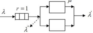
Figure 1. Two channel queueing system.
k=0 - there are no application in the system; k=1 - there is one application in the system;
k=2 - there is two application in the system; k=3 - there is three application in the system.
Figure 2. A marked transition graph. [3].
The formulas of necessary magnifications of M/M/2/1 system are shown in table 1.
Table 1. Mathematical characteristics of the M/M/2/1 system [1, 2].
Magnifications Formulas
Load y=λ/µ=λb
Utilization ρ=( 2 ∗ 2 ∗ )/2
Average number of working instruments k'=( 2 ∗ 2 ∗ )=2ρ
System idle ratio η= 1− ρ
Average number of requests in the queue l =
Average number of applications in the system m= 2 ∗ 3 ∗ = l+ k'
Probability of losing requests π=
The flow of served requests λ'=λ(1−π)
The flow of requests denied service λ''=λπ
Average waiting time of applications w= l/λ'
Average time of applications u= m/λ'=w+ b
Load is incoming flow. It is the average number of requests that arrive to the system. Utilization is attending to this incoming flow. Many packets can come in the system and total number of them is load. Utilization marks how to serve to them. For instance, in call center operators attend to subscribers. Whole number of subscribers are load. Utilization is probability of attending how many subscriber from whole ones. System idle ratio is reverse magnification to occupancy or utilization. It is the probability of making empty in the system. Average number of requests in the queue are packets which are waiting to be attended. It is set in the buffer. [5] Average number of applications in the system are collection of two packets. One of them is waiting to be attended. Next one is being served. Maximum occupancy is equal to one in M/M/2/1. Packet loss appears, in consequence of buffer size is limited. Probability of losing requests is probability which shows how many packets are lost. If it is considered to overhead example, sometimes operators cannot serve to subscribers. Served subscribers are as the flow of served requests. Ones who are not served, are look like the flow of requests denied service. Average waiting time of applications is subscribers’ waiting time in the queue. Average time of applications is collection of two times. First is subscribers’ waiting time in the queue and second is another’s served time in the server. [6]
Using formulas which is written in table 1, mathematical results are got. To find out load y, the values of average rate of packets and average duration of service requests must be given. They are selected voluntary. b is chosen only one value to make it as a permanent. λ is chosen four different
values to distinguish mathematical and imitation model. [7]
0.21, 0.45, 0.64, 0.81
Utilization ρ<1 for m-server in interval from 0.1 to 0.9. To calculate utilization values of , , are known. They are
found out using figure 2 (a marked transition graph). Incoming parameters are equalized to outgoing ones and formulas are written looking at , , , conditions. [4]
λ p μ;
λ p 2μ;
2 λ p 2μ;
2μ p λ;
, , are brought to formula which is found by and put to the following formula: 1 [8]
is found by overhead formula and also , , are known finding :
! ! !
" # "
(1)
$ %;
$! %!;
$"
%" (2)
Results of , , , are put in the formula of utilization and the state of , , , occupancy is calculated four times. Other magnifications are calculated by formulas shown table 1.
Table 2. Mathematical results of the the M/M/2/1 system.
Magnifications '( ). *( '* ). +, '- ). .+ '+ ). /(
Load, y 0.42 0.9 1.28 1.62
Utilization, ρ 0.2073 0.417 0.5473 0.638
Average number of working instruments, k' 0.4146 0.834 1.0946 1.276
Magnifications '( ). *( '* ). +, '- ). .+ '+ ). /(
Average number of requests in the queue, l 0.0121 0.073 0.1447 0.213
Average number of applications in the system, m 0.4267 0.907 1.2393 1.489
Probability of losing requests, π 0.0121 0.073 0.1447 0.213
The flow of served requests, λ' 0.207 0.417 0.547 0.637
The flow of requests denied service, λ'' 0.0025 0.0328 0.0926 0.172
Average waiting time of applications, w 0.0584 0.175 0.264 0.334
Average time of applications, u 2.0584 2.175 2.264 2.334
3. Results and Discussion
3.1. Imitation Model of the Intermediate Node
AnyLogic, is the standard in multimethod modeling technology, delivering increased efficiency and less risk when tackling complex business challenges. The unmatched flexibility found in AnyLogic allows users to capture the complexity of virtually any system, at any level of detail, and gain a deeper insight into the interdependent processes inside and around an organization. [9] AnyLogic includes a graphical modeling language and also allows the user to extend simulation models with Java code. The Java nature of AnyLogic lends itself to custom model extensions via Java coding as well as the creation of Java applets which can be opened with any standard browser. In addition to Java applets the Professional version allows for the creation of Java runtime applications which can be distributed to users. [12]
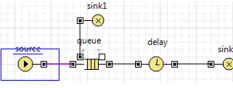
AnyLogic 6.4.1 software have been selected to create an imitation model of M/M/2/1. Imitation model includes following equipments:
Source object enerates entities with the specified interarrival time. Applications are objects that are produced, processed, serviced, or otherwise exposed to the simulated process: they can be customers in the service system, details in the production model, documents in the workflow model, etc. The queue object simulates the queue of clients waiting for maintenance. [10] The delay object models the delay. In an example, it spends a certain amount of time on customer service. The sink object indicates the end of the flowchart. Source, queue, delay and two sinks are chosen from enterprise library and they are connected to each other. [11]
Figure 3. Simulation model based on Anylogic 6.4.1.
Entities’ behavior can be defined by Java Class. Java Class named Modeling is established in the model.
Java class code
public class Modeling extends com.xj.anylogic.libraries.enterprise.Entity implements java.io.Serializable {
double a;
double b; double c; double d; double p; double plr; double l1; double l2; public Modeling () { }
public Modeling (double a, double b, double c, double d, double p, double plr, double l1, double l2) {
this.a = a; this.b = b; this.c = c; this.d = d; this.p = p; this.plr = plr; this.plr = l1; this.plr = l2; } @Override
public String toString () { return
"a = " + a +" " + "b = " + b +" " + "c = " + c +" " + "d = " + d +" " + "p = " + p +" " + "plr = " + plr +" "+ "l1 = " + l1 +" "+ "l2 = " + l2 +" ";}
private static final long serialVersionUID = 1L;}
Variables written in java class, are used to find values of M/M/2/1. [13]
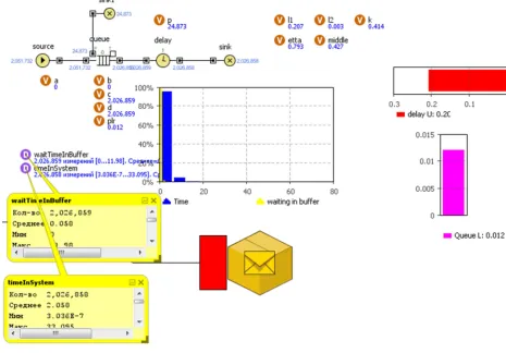
Values are entered in the source, delay and sink and the ready model is started up.
Figure 5. Simulation process in AnyLogic.
Values of , , , condition are entered and outgoing parameters are got.
Table 3. Imitation results of the M/M/2/1 system in AnyLogic.
Magnifications 0( ). *( 0* ). +, 0- ). .+ 0+ ). /(
Utilization, ρ 0.2 0.42 0.55 0.64
Average number of working instruments, k' 0.415 0.84 1.095 1.28
System idle ratio, η 0.793 0.58 0.453 0.36
Average number of requests in the queue, l 0.012 0.075 0.143 0.21
Average number of applications in the system, m 0.428 0.91 1.24 1.49
Probability of losing requests, π 0.012 0.08 0.169 0.27
The flow of served requests, λ' 0.207 0.414 0.532 0.591
The flow of requests denied service, λ'' 0.003 0.036 0.109 0.219
Average waiting time of applications, w 0.059 0.177 0.26 0.33
Average time of applications, u 2.064 2.18 2.266 2.33
3.2. Comparison the Imitation Model with the Mathematical Model Results
Using formulas, values of mathematical model has been detected. Imitation model has been built up, selecting objects in AnyLogic. The following table are shown, both mathematical and imitation model.
Table 4. Comparison model results.
Magnifications 0( ). *( 0* ). +, 0- ). .+ 0+ ). /(
Math. Imit. Math. Imit. Math. Imit. Math Imit.
Utilization, ρ 0.2073 0.2 0.417 0.42 0.5473 0.55 0.638 0.64
Average number of working instruments, k' 0.4146 0.415 0.834 0.84 1.0946 1.095 1.276 1.28
System idle ratio, η 0.7927 0.793 0.583 0.58 0.4527 0.453 0.362 0.36
Magnifications 0( ). *( 0* ). +, 0- ). .+ 0+ ). /(
Math. Imit. Math. Imit. Math. Imit. Math Imit.
Average number of applications in the system, m 0.4267 0.428 0.907 0.91 1.2393 1.24 1.489 1.49 Probability of losing requests, π 0.0121 0.012 0.073 0.08 0.1447 0.169 0.213 0.27
The flow of served requests, λ' 0.207 0.207 0.417 0.414 0.547 0.532 0.637 0.591
The flow of requests denied service, λ'' 0.0025 0.003 0.0328 0.036 0.0926 0.109 0.172 0.219 Average waiting time of applications, w 0.0584 0.059 0.175 0.177 0.264 0.26 0.334 0.33
Average time of applications, u 2.0584 2.064 2.175 2.18 2.264 2.266 2.334 2.33
Firstly, connection chart of magnifications are considered, to sum up looking at their connection. Then values of mathematical and imitation are compared, using bar charts.
Figure 6. Connection chart of load to utilization.
If flow enters to the system more, the occupancy of the queueing system rises as more as it. Despite the sharp increase in the load, utilization has gradually increased. When load is 0.42, utilization is equal to 0.2 it means, the incoming stream has been serviced with twice smaller probability. At the last point when load is 1.62, utilization is equal to 0.64 that is the incoming stream has been serviced with two and a half times smaller probability. The reason is arrival rate of packets are great values and service rate of the server has small value that is, identical to 0.5.
Figure 7. Connection chart of utilization to probability of losing requests.
As occupancy rises in the system, probability of losing requests goes up. At the beginning utilization is equal to 0.2, at this time probability of losing requests is equal to 0.012. ρ has a growth of twice greater value, it gets 0.42 value. At this time π gets six and a half times greater value relative to the initial state that is, 0.08. ρ has an increase of step by step after it has 0.42 value then it is equal to 0.64. At the end ρ
triples relative to the initial state, probability of losing requests has seven times greater value than the utilization. The reason is, maximum occupancy is limited, service rate of the server maintains the same level and it gets small one.
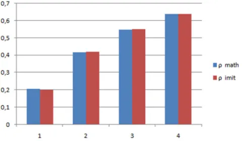
Figure 8. A bar chart of the M/M/2/1 system utilizations.
In this bar chart are shown, values of utilization in mathematical and imitation model are compared. When 1 is equal to 0.2073 in mathematical model, it gets 0.2 in imitation model. Mathematical value increased by 0.0073 compared to imitation value. When 1 is equal to 0.417 in mathematical model, it gets 0.42 in imitation model. Mathematical value decreased by 0.003 compared to imitation value. When 1 is equal to 0.5473 in mathematical model, it gets 0.55 in imitation model. Mathematical value declined by 0.003 compared to imitation value. When 1 is equal to 0.638 in mathematical model, it gets 0.64 in imitation model. Imitation value had a growth of 0.002 compared to mathematical value. The differences between mathematical and imitation values was less than 0.01.
Figure 9. A bar chart of probability of losing requests.
When 2 is equal to 0.0121 in mathematical model, it gets 0.012 in imitation model. Mathematical value climbed by 0.0001 compared to imitation value. When 2 is equal to 0.073 in mathematical model, it gets 0.08 in imitation model. Imitation value had a rise of 0.007 compared to mathematical value. When 2 is equal to 0.1447 in mathematical model, it gets 0.169 in imitation model. Mathematical value dipped by 0.0243 compared to imitation value. When 2 is equal to 0.213 in mathematical model, it gets 0.27 in imitation model. Imitation value increased by 0.057 compared to mathematical value. The difference between mathematical and imitation values was less than 0.06.
4. Conclusion
Modelling is for the process that would be controlled. It helps in understanding how the process would behave in various conditions. Modeling can reduce costs.
Queue is an important system not only in network, but also in other areas. If queue is organized properly, packet loss is reduced in telecommunication networks. Queueing system has been analyzed by two models. They are mathematical and imitation models. Both of them have their pros and cons. [14] Mathematical models can simplify a situation more complex, help us improve understanding of the real world as certain variables can be readily changed. But these models are a simplification of the real problem and does not include all aspects of the problem and they may only work in certain situations. If the situations changes, it has to calculated from the beginning. It takes lots of time. Imitation models can be useful even the state is changeable. This model also saves time as well as low cost. But finding out if the imitation model is working properly, it is had to develop a mathematical model. [15]
In this paper, queueing model which is based on Markovian process, number of servers and maximum occupancy are restricted, has been explained using mathematical and imitation models. Packet loss befall, in consequence of buffer size is finite. When mathematical and imitation model are compared, their values have been very
close together.
References
[1] Fundamentals of modeling discrete systems. T. I. Aliyev, St. Petersburg-2009.
[2] M. Guizani, A. Rayes Network Modeling and Simulation.- John Wiley & Sons Ltd, 2010.
[3] Michel C. Jeruchim Simulation of Communication Systems. – Nejw York, Kluwer Academic Publishers, 2002.
[4] K. Wehrle, M. Gunes Modeling and Tools for Network Simulation.- Springer-Verlog Berlin Heidelberg, 2010. [5] Jan Beran. Statistics for long-memory processes, chapter 12.
Monographs onstatistics and applied probability, No. 61. Chapman & Hall, New York, NY, USA, 1994.
[6] Brian D. Bunday, An Introduction to Queueing Theory- 1996. [7] Brian D. Bunday, Basic Queueing Theory-1986.
[8] Kamilov M. M. Ergashev A. K. Mathematical modeling.- Tashkent, TUIT, 2007.- 176 p.
[9] Krylov V. V., Samokhvalova S. S. Teletraffic theory and its applications. - SPb.: BHV-Petersburg, 2005. - 288 p.
[10] Vegeshna Sh., "Quality of service in IP networks" // Vestnik Svyazi, No. 1, 2008, M.: Williams Publishing House, 2003. [11] Zeliger N. B., Chugreev O. S., Yanovskiy G. G.
Proektirovanie setey i sistem peradachi disretnyx soobshchenie. -M.: Radio i svyaz, 1984.2.
[12] Kleinrok L. Teoriya massovogo obslujivani: Perg. s Ingliz. - M.: Mashinostroenie, 1979.
[13] Krylov V. V., Samoxvalova S. S. Teoriya teletrafika i ieo prilojeniya.- SPb.: BXV-Peterburg, 2005. - 288 s.
[14] Stepanov S. N. Osnovy teletrafika multiservisnyx setey.- M.: Eco-Trends, 2010.- 392 s.