~ 288 ~ WWJMRD 2017; 3(8): 288-298
www.wwjmrd.com International Journal Peer Reviewed Journal Refereed Journal Indexed Journal UGC Approved Journal Impact Factor MJIF: 4.25 e-ISSN: 2454-6615
Bekir Cirak
Siirt University, Engineering & Architectural Faculty, Department of Mechanical Engineering, Kezer Campus, Siirt - Turkey
Correspondence: Bekir Cirak
Siirt University, Engineering & Architectural Faculty, Department of Mechanical Engineering, Kezer Campus, Siirt - Turkey
MPC controller used with ARX methods via control
and modelling with ANN for a wire coating thickness
Bekir Cirak
Abstract
Nowadays, wire coating process is used in almost every area especially in the electrical and electronic industry. Wire coating is a process which utilizes a variety of complex equipment. This consists of a plasticating extruder fitted with a wire coating die through which the wire is continuously drawn. A three layer back propogation artificial neutral network (ANN) model was used for description of wire coating thickness. On comparing the experimental data, the predictions the ANN model predictions, it is found that the ANN model is capable of predicting the coating thickness. In this paper, the results of experimental investigation are presented by comparing the coating quality on galvanized mild steel wire using EP 58 PVC molten is used as the coating material in a wire coating extrusion unit at different extruder temperatures and extruder speeds.
Simulations of MPC Control algorithms for coating process have been made and the results of these simulations was observed. There are a comparison of PID Controller and Generalized Predictive Controller results and there are comments about this comparison in these studies. The simulations and calculations of the algorithms are done in MATLAB Packaged Program Environment.MPC is especially suitable for controlling these types of systems. MATLAB Packaged Program is utilized in all these studies.
Keywords: Wire coating Processes, Coating thickness, artificial neural network PVC, Matlab Extrusion, Model Predictive Control
Introduction
Polymer coating is often applied to wires, strips, tubes or ropes for insulation or protection against corrosion. There are three different methods which are mostly used for this coating process. These methods are coaxial extrusion, dipping and electro-statical deposition process. The first two processes can be reasonably fast but bonding between the continuum and the coating material is not so strong. The third process offers much stronger bonding but is relatively slow. If the coating material can be forced onto the continuum uniformly the bonding can be improved significantly. The analysis for different coating processes could be found in the literature. Hydrodynamic wire coating with Nylon 6 using a tapered bore pressure unit was presented. in Ref. [1. In Refs. [2–5]], coextrusion method for coating were studied theoretically and experimentally.
Nomenclature
SSE Single screw Extruder PVC Polyvinyl chloride ANN Artificial Neural Network MPC Model Predictive Control SISO Single Input Single Output ARX Auto Regressive with eXogenous
Refs. [6,7] present studies of dip coating process. An experimental study of the electro-statical deposition process were presented in Ref. [8]. A continuously increasing number of commercial products are produced by polymer extrusion using plasticating extruders, which are among the most widely used equipments in polymer process industry. The extrusion process has a standard setup including a feeding section, a barrel and a head with a die for
shaping. In the feeding section, the solid polymer is fed into the extruder through a hopper in the form of pellets or irregular small bits. Then, the polymer is transported along the barrel by means of a rotating screw.
The plasticating extruder is one of the main pieces of equipment used in the polymer processing industries. As plastics are found more uses, with more stringent quality specifications, the methods of increasing polymer production while improving product quality are needed. Extrusion molding is the most widely used process in manufacturing plastic products. Since the quality of extrusion coated plastic parts are mostly influenced by process conditions, how to determine the optimum process conditions become the key for improving the part quality.
Material and experimental procedure
In this study, EP 58 PVC coating plastic material was used as test material. The material was supplied from EL-Kİ KABLO (Manisa/Turkey). The experimental value and data
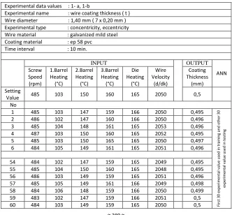
is given from this company. The die heating zones was maintained at the same temperature, which was also varied during the experiments. Some of temperatures for each heating zone (barrel) and the different screw speeds are shown in Table 1. Sixty combinations were tested for their effect on the parameters of the extruded parts. The process settings were varied randomly and continuously; i.e. without stopping the process. Each setting was allowed to run. Table 1 shows first 30 experimental values used in training and used in testing.Total values used 60 piece. To measure the coating thickness, each sample was measured at five different positions along its length by a micrometer and the average diameter of the coated wire is noted. A small portion of the wire sample is cold mounted and is polished. An optical microscope is then used to assess the actual coating thickness and the concentricity of the coating on the wire. Fig.1. shows geometry model of coating thickness and this model to consist of an optical microscope.
Fig. 1: Coating thickness geometry model
The geometry gives distance of coating centre between wire centre of wire coating section. In this paper, the wire coating states of an industry example. The polymer material used for coating the cover is PVC. Also the geometry gives distance of coating center between wire center of wire coating
section. The other words, the eccentricity (uniformless coating) and concentricity (uniform coating) of the wire coating states of an industry example, shown in Fig.1 was studied.
Table 1: Range of experimental process parameters
Experimental data values : 1- a, 1-b
Experimental name : wire coating thickness ( t ) Wire diameter : 1,40 mm ( 7 x 0,20 mm ) Experimental type : concentricity, eccentricity Wire material : galvanized mild steel Coating material : ep 58 pvc
Time interval : 10 min.
INPUT OUTPUT ANN Screw Speed (rpm) 1.Barrel Heating (°C) 2.Barrel Heating (°C) 3.Barrel Heating (°C) Die Heating (°C) Wire Velocity (d/dk) Coating Thickness (mm) Setting
Value 485 103 150 160 165 2050 0,5
No
1 485 103 147 159 166 2050 0,495
Fi rs t 3 0 ex p er imenta l v al u e u sed in t rai n in g an d o th er 3 0 ex p e ri menta l v al u e u sed in t es ti n g
2 486 102 147 160 166 2050 0,496
3 485 104 148 161 165 2053 0,496
4 487 103 150 160 165 2052 0,495
5 485 103 150 165 165 2050 0,497
6 484 105 149 161 165 2051 0,496
54 484 102 147 159 165 2049 0,495
55 485 104 150 160 165 2048 0,495
56 486 103 149 159 165 2051 0,496
57 485 105 149 161 166 2049 0,498
58 484 106 148 159 166 2050 0,499
59 483 102 147 159 166 2051 0,5
~ 290 ~
The coating concentricity at extruder temperature 175 ◦C and wire velocity of 19 m/s which appears to be slightly eccentric. The coating is reasonably concentric. Results the quality of concentricity of the coating on wire with extruder temperature 150 ◦C and wire velocity of 15 m/s. However, the coating on the polymer for different ranges of velocities, and extruder temperatures appeared to be concentric. Some samples were prepared and polished for examination under an optical microscope. The cross section of the wire was observed to be circular and the coating was reasonably concentric.
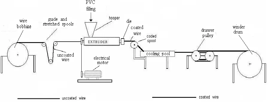
The experimental set up consists of the drawing bench, the
wire bobbine, the cooling pool, the drive system (electrical motor), the polymer feeding and melting unit (extruder) and the drawer and winder unit. A schematic diagram of the process is shown in Fig. 2. The polymer granules are filled in the hopper and the hopper is connected to the body of extruder.
PVC is extruded using a laboratory scale co-rotating single screw extruder (SSE, L/D=24) The schematic drawing for the extruder system is given in Figure 2. The extruder had five electrical heaters through the barrel, whose temperatures can be set separately.
Fig. 2: Wire coating extrusion process scheme
The cooling is provided by passing through cooling water in the barrel. The available measurements from the control panel are screw speed, temperatures of each three heating zones, wire velocity and die temperature from four distinct points. The process parameters for the investigations carried out were as follows. Polymer characteristics Polymer type EP 58 PVC, Polymer melt temperature 150–200 ◦C and Wire characteristics; Wire diameter 1,40 mm (0.20x7 mm), Wire material, Galvanized mild steel. Experimental work was carried out at polymer melt temperatures of 150, 185 and 200 ◦C.
A PVC compound was prepared using a proprietary formula which includes PVC
resin, foaming (blowing) agent, heat stabilizer, lubricant, process aid, and filler. The
extrusion process parameters; i.e. barrel heating zones’ temperatures and screw speed were
varied systematically and in random order to vary of the extruded parts [9].
The available extruder incorporated three heating zones along the barrel and two
independent heating zones at the die sections. In order to maintain a constant heat profile in the barrel, the ratio between the three heating zones was fixed during all experiments while varying the temperatures of all three barrel zones accordingly.
Artificial neural networks
In recent years artificial neural networks (ANNs) have emerged as a new branch of computing, suitable for applications in a wide range of fields. Artificial neural networks have been recently introduced into plastic extrusıon [10]. In this study, experimental and ANNs results have been compared. A lot of studies have been published in
which the prediction of various parameters on coating thickness were investigated systematically.
Structure of an ANN model for coating thickness
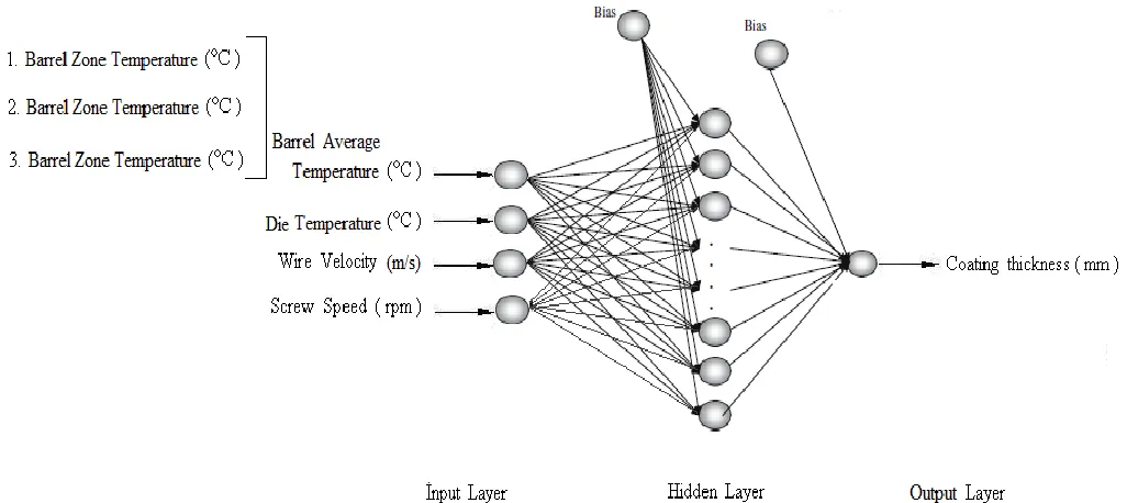
In this paper, the selection of process variables as inputs of ANN model is based on the relative significance of each variable on the objective performance. The neuron number of the input layer of ANN is determined by the number of variables selected, and the neuron number of the output layer is determined by the number of the objective indexes. Many different process parameters affect the quality of the injection molded products. Variables with greater influence on the part quality need to be selected in order to simplify the problem by saving both the sample collecting time and the computing time. In this paper, a three-layer ANN model with one hidden layer was used, where the neuron number of the hidden layer was determined by trials. The transfer function between the input layer and the hidden layer is ‘Tansig’, while the transfer function between the hidden layer and the output layer is ‘Purelin’. The architecture of a neural network depends on its network topology, transfer function, and learning algorithm. A typical Back-propagation neural network, as shown in Fig. 3, is composed of three layers, namely, input layer, hidden layer, and output layer [12].
ANNs are widely accepted as a technology offering an alternative way to simulate complex and ill-defined problems. They have been used in diverse applications in control, robotics, pattern recognition, forecasting, power systems, manufacturing, optimization, signal processing, etc., and they are particularly useful in system modeling. A neural network is a computational structure, consisting of a number of highly interconnected processing units called neurons. The neurons sum weighted inputs and then applies a linear or non-linear unction to the resulting sum to determine the output and the neurons are arranged in layers and are combined through excessive connectivity [12]. Back propagation network is a typical ANN that has been widely used in many research fields. Back propagation network have hierarchical feed forward network architecture, and the outputs of each layer are sent directly to each neuron in the layer above. Back propagation network are trained by repeatedly presenting a series of input/output
pattern sets to the network. The neural network gradually ‘learns’ the governing relationship in the data set by adjusting the weights between its neurons to minimize the error between the actual and predicted output patterns of the training set. A separate set of data called the test set is usually used to monitor network’s performance. When the mean squared error (MSE) of the test set reaches a minimum, network training is considered complete and the weights are fixed. In essence, a neural network is a function that maps input vectors to output vectors [13].
In this work, a back propagation neural network model was developed to build the relationship between parison thickness distribution and the objective function. The thicknesses of 0.5 mm positions arranging uniformly along the parison were selected as input parameters for the ANN model. The output parameter was the objective function value. The architecture of a neural network depends on its network topology, transfer function, and learning algorithm. A typical back propagation neural network, as shown in Fig. 4, is composed of three layers, namely, input layer, hidden layer, and output layer. There is no definite rule available to determine the appropriate number of neurons in the hidden layer. In this paper, it was determined by a trial and error method. The results showed that the ANN model with 13 neurons in the hidden layer could give a better converging rate and generalization. The architecture of the ANN model used in this work is shown in Fig. 4.
The ANN model for the coating thickness variation of the part built by the above methods is shown in Fig. 4. The node number of the hidden layer was determined by train trials and the final value obtained was 9, that made the configuration of ANN as 4–9–1. A neural network system is presented for use in wire coating process. The tan-sigmoid transfer function was used as the activation function for the hidden layers, and linear transfer function was used for the output layers. Network architecture for coating thickness and the contrast of prediction results and numerical experiment results of relationship between coating thickness variation and process parameters are shown in Fig. 3.
~ 292 ~
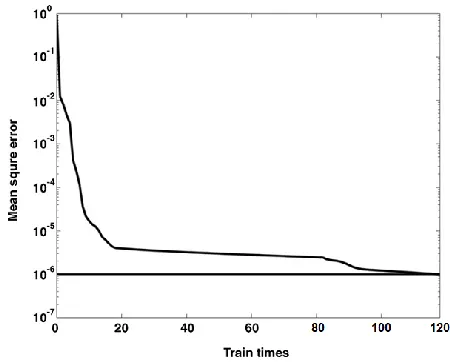
Among them, 30 patterns were used as training ones. Once the mean square error (MSE) for the training patterns reduced within the number of training iterations reached a predetermined one (set at 1000 in thiswork), the network-training course was stopped.Fig. 4 shows iteration number versus mean square error for training nonlinear coating thickness.
Fig. 4: Iteration number versus mean square error for training nonlinear coating thickness
The results of training and testing are confirmed experimentally. According to the back propagation models, the R2 for training and for testing is 0.924 and 0.822,
respectively, which means that the experimental hardfacing roughness values and their predicted values are strongly linear for both models. The values predicted by the back propagation model analysis yield a best-fit average percentage error of 4.61% from the actual data. Figs.5 show the development of training and testing RMS errors for 10,000 learning epochs.
Fig. 5: The development of training and testing RMS with learning epochs fort he 4-9-1 ANN model
The 4-9-1 neural network models, which exhibit well-trained network performance, are superior to the other networks used because the RMS errors for training and testing are
rapidly minimized, converging to 0.035 and 0.061 following after 4400 learning epochs, respectively.
Fig.6 shows the evolution of the mean square error of the ANN model during training. The trained network model was validated for its predictive capability.The result indicates that the ANN has a good performance graphics in Fig.6
Fig. 6: Train error during the training
Train/test samples
This paper deals with the ability of the varied step of each variable is set to obtain a series of set point values of variables inside the varied range based on baseline. The samples of all set-points are then assigned as input–output data to train and test the ANN. The samples are randomly divided into two groups. Those samples including the baseline set were methodically assigned to the training set, and all the remaining samples were assigned to the test set. After being trained, the ANN model can map the non-linear relationship between input variables and variables of coating thickness. It can then be used in the optimization of online process conditions and the part quality control of molded products.
The simulation function based on the ANN was used as the objective function of the optimization problem, and the process window for each variable as given above was used as the boundary restrictions. The remaining 89 samples were then used to test and to train the performance of the ANN. As shown in Fig. 7,8 most of the samples have consistent outputs of ANN prediction and numerical experiment, and the result is quite satisfactory.
Fig. 8: Plant and model responses to a unit step changes in test samples
The number of the hidden layer with 18 neurons is obtained from Table 2. Table 2 reveals that the suitable number of neurons in the hidden layer is determined by trial and error. However, 11 neural network constructs are obtained using
the MATLAB1 interface. The 4-9-1 and 4-13-1 neural models both have small and stable RMS errors for various constructs, respectively.
Table 2: The various RMS errors of ANN models through learning epochs
Trials Number İnput-hidden-output neurons RMS error of training samples RMS error of testing samples 1
2 3 4 5 6 7 8 9 10 11
4-8-1 4-9-1 4-10-1 4-11-1 4-12-1 4-13-1 4-14-1 4-15-1 4-16-1 4-17-1 4-18-1
0.03378 0.03378 0.03378 0.03377 0.03377 0.03377 0.03381 0.03379 0.03377 0.03378 0.03379
0.0605 0.0619 0.0699 0.0654 0.0645 0.0656 0.0610 0.0661 0.0672 0.0669 0.0665
Model Predictive Control
Model Predictive Control (MPC) is commonly used for control of highly stochastic processes where selection of control actions, based on optimization, is desired. The importance of MPC compared with traditional approaches is due to its suitability for large multi-variable systems, handling of constraints placed on system input and output variables, and its relative ease-of-use and applicability. In MPC, current and historical measurements of a process are used to predict its behavior for future time instances. The MPC is supported by commercial tools such as MATLAB (Mathworks 2010a).
It consists of a System Prediction Model and Optimizer. The error between future outputs and target trajectories (i.e., expected customer demand) is sent to the optimizer where optimized control outputs (referred to as manipulated variables) are calculated based on some constraints and
objective functions over some time horizon-i.e., moving horizon (for manipulated variables) and prediction horizon (for controlled variables). This optimization will be repeated using the receding horizon concept once the new information is available. In addition, the MPC has a filter gain that can respond quickly to inevitable signal to noise ratio changes while avoiding undesirable oscillatory control regimes. The predictive control for the first time step is sent to simulated system as well as the system prediction model. The above steps are repeated using the updated simulated system states and disturbances for a desired simulation period.MPC is not a specific control strategy but a wide class of optimal control based algorithms that use an explicit process model to predict the behavior of a plant. There is a wide variety of MPC algorithms that have been developed over past 30 years [14].
~ 294 ~
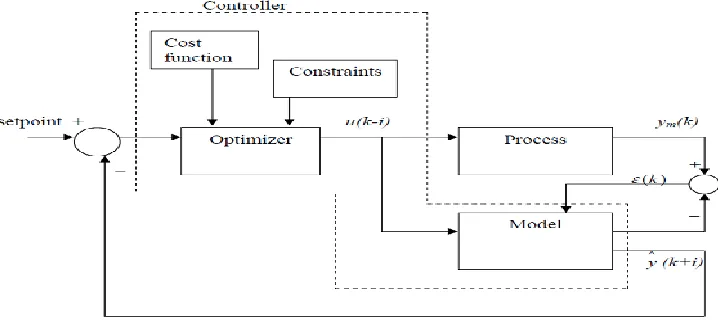
The basic elements of MPC are illustrated in Figure 9. and can be defined as follows:
1. An appropriate model is used to predict the output behavior of a plant over a future time interval or normally known as the prediction horizon (P). For a discrete time model this means it predicts the plant output from ŷ(k +1) to ŷ (yk+ H p) based on all actual
past control inputs u(k), u(k −1),..., u(k − j) and the available current information y(k).
2. A sequence of control actions adjustments (Δu(k/k-1)…
Δu(k+m/k-1)) to be implemented over a specified future time interval, which is known as the control horizon (m) is calculated by minimizing some specified objectives such as the deviation of predicted output from setpoint over the prediction horizon and the size of control action adjustments in driving the process output to target plus some operating constraints. However, only the first move of computed control action sequence is implemented while the other moves are discarded. The entire process step is repeated at the subsequent sampling time. This theory is known as the receding horizon theory [15].
3. A nominal MPC is impossible, or in other words that no model can constitute a perfect representation of the real plant. Thus, the prediction error, ε(k) between the plant measurement y(k)m and the model prediction ŷ(k) will always occur. The ε(k) obtained is normally used to update the future prediction. The Figure M. illustrated the error feedback of MPC.
Sistem identification
Identification of the system used Matlab 2010a toolbox to creat a model program in MPC control, again by using Matlab 2009b-toolbox system for modelling.MPC occured by plant model enviroment. ARX and ARMAX models are used.For preparing of models, linear parametric models are satisfied by MATLAB System Identification Toolbox 7.9. System models are lineeralized by basic polinomal equations (4.1.) (4.2.) (4.3.) (4.4.) and (4.5.).
A(q) =1+a1.q−1 + _ _ _ + ana.q−na (4.1.)
B(q)=b1.q−1+_ _ _+bnb.q−nb (4.2.)
C(q) = 1+c1.q−1 +_ _ _ + cnc.q−nc (4.3.)
D(q) = 1+d1.q−1 + _ _ _ + dnd.q−nd (4.4.)
F(q) = 1+f1.q−1 + _ _ _ + fnf.q−nf (4.5.)
Therefore
na : model for y (t), how much (t) quantity is added by A
polinomial parameter.
nb : model for u (t), how much (t) quantity is added by B
polinomial parameter are explained the degree of models.
nk : shows between input-output lates models parameters.
Than these polinomials, Equations (4.5.) is inserted. Models are designed by SID (System Identification) for linear equations structure, is shown by (4.6.) There are several different model structures which tie in with the above postulate. A quite general structure is
A(q) y(t) =B(q)
F(q)u(t) +
C(q)
D(q) e(t) (4.6.)
Equations (4.6.) is shown Parameters are determined (q), slide operator, y ( t ) output, u ( t ) input, e ( t ) errror, t
illustrate times. A (q ) and B (q), C(q), D(q), F(q), q depend on operator polinomals [16]. One of the simplest and most common model structure used is the (AutoRegressive with eXternal input) structure,
𝑦(𝑡) =𝐵(𝑞)
𝐴(𝑞) 𝑢(𝑡) +
1
𝐴(𝑞) 𝑒(𝑡) (4.7.)
As can be seen from (4.7) this is the same as (4.6) using C(q) = D(q) = F(q) =1. ARX model linear polinomal equations is calculated for coating thickness protype model by used benefical simulation.
A(q)= 1− 0,3055 q-1 + 0,2457 q-2− 0,1536 q-3(4.8.)
B(q)= 0,2471 q-4
− 0,09878 q-5 (4.9.)
MPC control model inner system for ARX model, taken from system and non-linear data linearized by equations of (4.8.) and (4.9.) for thickness model. Linear model output values, approximately equals to real results and benefit to curve at Figure 10. ARMAX and ARX models outputs and process real data are showed at Figure 10 by comparing each us. ARMAX and ARX models by using experimental results which is fitted at 89,10% ratio to ARX models. ARMAX model is fitted at 51.08% ratio.
Fig.10: ARX and ARMAX model responses to unit step changes in thickness
In order to generate a step response process model that can be used in MPC algorithm, ARX models are formulated and used to obtain the thickness response to a step change in
MPC methods is developed for optimiztion; is very important topic. If criterion square is depended on by inputs and outputs solutions, linear function is explained. If tere are no constratied valus, by using iteractive approach for solving the problems which is the methods long [16].
There are a large amount of different parameters available for tuning in the combined problem of system identification (sıd) and (mpc) predictive control. Those which relate to system identification and to predictive control see Table 3.
Tabel 3: SID and MPC tuning parameters
Parameters Definition Value
N2 Length of prediction horizon 10
NU Length of control horizon 1 2 3
na Exponantional of the A polynomial 1 2 3
nb Exponantional of the A polynomial 1 2
nc Exponantional of the A polynomial 1
nk Delay of model 1
TS Sample numbers 0.001
Feedback control loop for PID controllers designed in SIMULINK. PID control loop designed using SIMULINK
is given in Figure 11.
Fig. 11: PID Control Model by Simulink
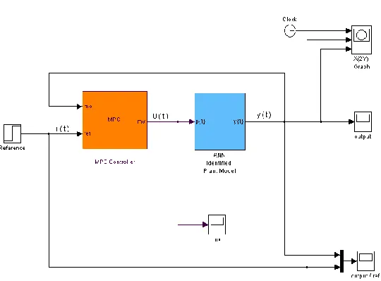
Feedback control loop for MPC controllers designed in SIMULINK. MPC control loop designed using SIMULINK
is given in Figure 12.
Fig. 12: MPC Control Model by Simulink
PID Control
PID controllers are used in the designed control system. PID controllers are designed usingthe convolution models of the
~ 296 ~
The fine tuned PID control parameters KP = 0.2948, KI =
0.1275 and Kd = 0.3925 are accepted.These PID settings are
very small and cannot be implemented on a nominal operating industrial plant controller.However, if a computer is used for the PID controller, then these settings can be implemented. Therefore in this study for comparison with the MPC, also placed on PID outputs thickness to be able to compare PID controller with the MPC. In the design and testing of Model Predictive Control MPC as for PID
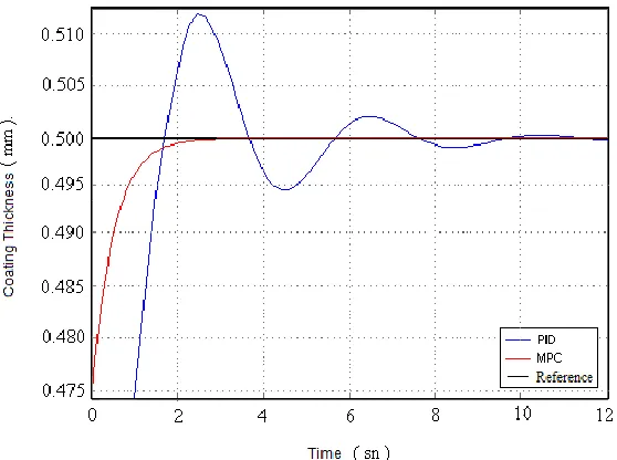
controllers, two parallel working SISO MPCs are constructed using the model predictive control toolbox of MATLAB, for non-linear constrained MPC.Examine of Figure 13 by model controler at first 3 seconds, prcoses responds 0.500 mm valued by PID controler to maximum value 0.512 mm. Model.esponded to PID controler very quickly. All of controler for coating thickness is accepted under fix references value of 1% error.
Fig.13: Comparison of MPC and PID results (ref = 0.500mm)
As can be seen at Figure 14 in references to the variable that is running under the process of MOK, and PID control with the MPC there is a distinct difference between the answers of a more rapid response than the PID controller are given. MPC-line method, the reference value of thickness of less
than 1% error with a permanent error with PID control method, permanently settled in around 1%. Describes the model predictive controller has a faster response than PID controller.
Fig.14: Comparison of MPC and PID results (ref=0.500mm-1mm-1.5mm-0.400 mm)
As a result of all this work 5% error rate remaining below the thickness of the wire coating industry, and literature are acceptable for the exchange of values is taken into account that the model predictive controller was developed to be reliable, the simulation results and performance of the best in the industry as well understood. As is clear from here the
model predictive controller has a faster response than PID controller.Others studies in the literature, other MPC controller according to conventional controllers, and PID controller show that a new controller [16].
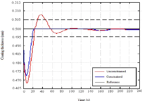
conditions for the simulations were defined.Constraints identified for wire coating system. First, the control signals applied to the maximum and minimum values of the DC motor and extruder temperature (0-10 V, which corresponds)
to 147-176 ° C and the constraints defined in system.The constrained and unconstrained responses of MPC controller show in Figüre 15.
Fig.15: Comparision of constrained and unconstrained MPC controller response
Figure 15. describes the unconstrained state has been % 6 pick after % 1.8 error and sit in 180 oC. Although the constrained state has been % 1 pick after % 1error and sit in 180 oC.
The system has a structure that the constraints too. This control system, makes it difficult to be made with the classic multi-variable control algorithms. The results from this simulation and the curve has been controlled successfully against the constraints of the mpc.
Conclusion
In this study, experimental and theoretical studies are done to design an inferential control
scheme for the feedback control of wire coating thickness during polimer extrusion process. The basic conclusions arrived are as follows:
This paper is presented knowledge based and neural network approaches to wire coating for polymer extrusıon. Experimental results of wire coating extrusıon with EP 58 PVC have been presented. Due to some limitation in the present experimental set up the drawer speed is limited to about 16 m/s. Therefore, experiments were carried out within the speed range of up to 15 m/s. The polymer coating on the wire is continuous for speeds of up to 15 m/s The bonding quality of the coating with wire was found to be very good. Concentricity is beter in the case of extruder with screw speed 485 rpm and wire velocity 2050 rpm (15 m/s) Application of screw speed and wire velocity (drawer speed) generally improves the quality of the coating. Conventional wire coating with EP 58 PVC using a tapered bore die unit has been presented. The experiments were carried out within the speed range between 2 m/s and 15 m/s The polymer coating on the wire is continuous and concentric for speeds of up to 16 m/s The concentricity quality of the coating with wire was very good.
For the two controllers designed, the analyses for robustness should be carried out also, in order to compare the controllers in this scope, which is also veryimportant. Next to this, accomplishing comparisons of the results of the two
controllers which are included in the nonlinear model, but the effects are not investigated. Additionally, carrying out the real time applications by first discretizing the controller developed in this study, which are continuous, may be considered as a possible future work.
Coating thickness of 0,495 mm - 0,505 mm in the range selected for the simulation of the system if it is controlled by PID controller, while exceeding the 5.8% of the exceedance, when controlled by the model predictive controller was observed to be 2%. However, the value of thickness of the PID controller, a 5% error with the reference model predictive controller 1.8% error with the reference placed settled.
As a result, the model predictive control (MPC), the desired wire coating system is controlled within acceptable limits. Compared with PID controllers, PID controller, MPC observed that the control system, such as variable references under the system successfully. However, given the restrictions on the model predictive controller based PID controller concluded that a more healthy work
Suggestion
The system, in addition to the variable thickness of the coating surface quality of coating can be controlled in a structure can be converted to variables. In this way, input increasing the number of output, the control problem becomes a bit more complicated. Example, the viscosity and shear rate (flow rate) variables, with the participation of the system against the performance of predictive control algorithm is the effect of dead time, can be tested.Viscosity and shear rate for the coating surface quality control concepts can be examined, and these concepts can be done to improve the quality of the surface.
References
~ 298 ~
2. Ozbek M. O., Inferentıal Model Predıctıve Control of Polyethylene terephthalate Degradatıon Durıng Extrusıon, The Graduate School of Natural and Applıed Scıences of Mıddle East Technıcal Unıversıty, 56, 2006, ( 25-34).
3. Schön T., Identification for Predictive Control-A Multiple Model Approach, Master's Thesis, Division of Automatic Control Department of Electrical Engineering, Link¨oping University, 54, 2001, ( 45-52). 4. Der Jean M., Du Liu C., Ting Wang J., Design and development of artificial neural networks fordepositing powders in coating treatment, applied surface science, Computer Science, and Statistics, State University, 69, 2005, (290- 303).
5. Qun Huang G., Xiong Huang H., Optimizing parison thickness for extrusion blow molding by hybrid method, Journal of Materials Processing Technology, 51, 2007, (512-518).
6. Changyu S., Lixia W., Qian Li., Optimization of injection molding process parameters using combinationof artificial neural network and genetic algorithm method, National Engineering and Research Center for Advanced Polymer Processing Technology, 36, 2007, (412-418).
7. Nidal H. Zahra A., Seth A., In-process density control of extruded foam PVC using wavelet packet analysis of ultrasound waves, Industrial and Manufacturing Engineering Department, University of Wisconsin-Milwaukee, 90, 2002, (1083-1095).
8. Durmus H. K., Ozkaya E., Meric C., The use of neural networks for the prediction of wear loss and surface roughness of AA 6351 aluminium alloy, Department of mechanical engineering, Celal Bayar University, 32, 2004, (201-205).
9. Caswell B., Tanner R.I., Wire coating die design using finite element methods, Journal Polymer Engineering Science, 18, 1978, (417-421).
10. Han C.D., Rao D., Studies on wire coating extrusion.1.The rheology of wire coating extrusion, Journal Polymer Engineering Science, 40, 1978, (1019-1029).
11. Basu S., A theoretical analysis of non isothermal flow in wire coating co extrusion dies, Journal Polymer Engineering Science, 21, 1981, (1128-1137).
12. Zhang H., Moallemi M.K., Kumar S.,Thermal analysis of the hot dipcoating process, journal of heat transfer in metals and container less processing and manufacturing, ASME, 21, 1991, (49-55).
13. Nakazawa S., Pittman J.F.T., A finite element system for analysis of melt flow and heat transfer in polymer process, in: Numerical Methods in Industrial Forming Process, Pineridge Press, Swansea, 57, 1982, (523-533). 14. Cirak B., Kozan R.,” Prediction of the Coating Thickness of Wire Coating Extrusion Processes Using Artificial Neural Network (ANN) ”, Journal of Modern Applied Science,Vol 3, No 7, pp. 52-66-Jully 2009 15. Kuhl M. E., Steiger N. M., Armstrong B. F., Joines J.
E., Hybrıd dıscrete event sımulatıon wıth model predıctıve control for semıconductor supply chaın manufacturıng, Arizona Center for Integrative Modeling and Simulation Control Systems Engineering of the laboratory proceedings. 61, 2005, (112-120).