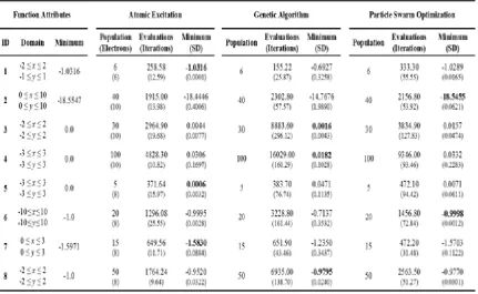
ISSN (e): 2250-3021, ISSN (p): 2278-8719
Vol. 06, Issue 12 (December. 2016), ||V1|| PP 05-17
Optimization through an Atomic Excitation Model
Mateus de Araujo Fernandes
11(Federal Institute of Education, Science and Technology in Sergipe, Aracaju/SE, Brazil,)
Abstract: - This paper intends to introduce a new metaheuristic, designed to solve optimization tasks. The proposed algorithm is a population-based neighborhood search inspired by a simplified atomic excitation model, where the energy state of an atom has influence in its orbital radius (region around the atom’s nucleus with probability of finding electrons). An initial population of atoms is distributed in the search space, evaluating the cost function – which here mimics the energy level – at their nuclei’s positions and with this establishing the surrounding space that will be investigated by the electrons that orbit each atom. The cost function evaluation performed by these electrons then dictates the new positions for their respective nuclei, with this initiating the next iteration in a process that is repeated until the convergence criteria are reached. The algorithm was tested using some benchmark functions indicated in the literature and then compared with other population-based methods, showing a superior overall performance while finding successfully the functions’ minima with fewer evaluations and, consequently, with an inferior computational cost.
Keywords: - Combinatorial optimization, Metaheuristics, Neighborhood Search, Population-based algorithms.
I.
INTRODUCTION
Optimization, initially conceived as the simple act of finding the minimum (or maximum) value of a function, long ago left behind this simplistic vision to become a multidisciplinary and increasingly important field of study. With a huge amount of problems – not only related to engineering – consisting in minimizing disadvantages and costs, maximizing quality and profits, or determining optimum operating points for systems and processes, optimization can nowadays be considered as one of the study areas of greater scope in the technical-scientific world.In the middle of the current effervescence in the studies of new optimization methods, this work presents a novel population-based and nature-inspired metaheuristic: the Atomic Excitation model (AE). The optimization algorithm proposed relies on an initial population of atoms randomly distributed around the search space, for which the cost function is evaluated at the position corresponding to their nuclei. Based on the values obtained – corresponding to energies or excitation levels of the atoms – the radii are established for the investigation to be held by their respective “electron clouds”, dictating this way the nuclei’s positions in the following iteration. This process is then repeated in order to obtain the lowest and more stable energy state, until the convergence criteria are met.The present work has its forthcoming sessions organized as the following description. After this Introduction, Section 2 presents a brief review of the pertinent literature, showing synopses of some of the most prominent optimization metaheuristics. Section 3 provides a brief description of the development of atomic theory, starting from its primordium and reaching the current stage, including the quantum modeling with its ground and excited states, that is the source of inspiration for this work. Afterwards, Section 4 presents the general characteristics, the implementation details and the particularities of the algorithm developed. The subsequent Section 5 shows the results obtained by the Atomic Excitation model in optimizing some benchmark functions found in the literature, designed exactly for the purpose of testing the performance of optimization methods. These results are compared to those obtained for the same functions by means of a Genetic Algorithm and a PSO. Finally, Section 6 brings the final discussions and the concluding remarks.
II.
REVIEW
ON
METAHEURISTIC
ALGORITHMS
Although mathematical optimization methods are being studied for centuries (the renowned Newton’s method, for example, dates back to the seventeenth century), the evolution of computer technology over the last decades has boosted the development and enhancement of a wide variety of methods and algorithms.
computational cost when these methods are compared to deterministic ones (derivative-free or not), due to the higher required number of objective function evaluations [3].The multidisciplinary approach is a hallmark of the metaheuristics, leading optimization to transcend the areas of mathematics, computer science and operations research while finding sources of inspiration for algorithms in areas such as biological and even social sciences. These metaheuristics can be based on trajectories or, more commonly, populations [4], where the optimization process’ concern is to improve, after each iteration, the overall performance of a group of individuals. Different approaches to promote improvements in each step originate different families of methods, and among those, the evolutionary and swarm intelligence algorithms are foregrounded because of recent advances. In the following paragraphs, some highlights from these families of methods are reviewed.The Simulated Annealing is considered to be the first metaheuristic, dating from the early 80’s with the works by Kirkpatrick et al. and Cerny [apud 4]. The method is based on the tempering process, in which a material is melted and, in the sequence, passes through a cooling with controlled temperature so that at the end of the procedure this material is in a crystalline lattice, with lower energy, that here is the analogous of the cost function. When the temperature is high, evaluations at points farther away from the current are permitted, and there is a greater probability of acceptance of a result worse than the actual, which is the key to the algorithm to escape from local minima. As the temperature is reduced, this flexibility also is, resulting in the convergence [3].
The Genetic Algorithms (GA) pioneered the Evolutionary Algorithms and, until nowadays, it is perhaps the most prominent expression of this family of metaheuristics, with an infinity of different applications, diverse useful adaptations and integration with other computational methods. Its operation is based on the concepts of natural selection and evolution, where a population of chromosomes, each of them being associated with a point in the search space, evolves over several generations through the exchange of characteristics among themselves [5]. For this end, the best-fitted individuals are more likely to be selected for the crossover operations. At the same time, mutations are responsible for inserting a larger amount of randomness to the process. An important feature of the method is to prioritize the improvement of an entire population, at the expense of concerning about individual performances at each iteration [3].
Another population method, but introducing a different approach, is the Particle Swarm Optimization (PSO), that makes use of a mix of models of artificial life and evolutionary computation to generate a “swarm intelligence” [6]. In this method, individuals wander through the search space with movement governed by a combination of randomness and attraction to the direction of the best momentary evaluation, what results in a robust and efficient optimization method.The success of these groundbreaking metaheuristics incited studies in order to develop new methods inspired by nature, whether in its physical processes or populations’ behavior. Belonging to the first group, the Gravitational Search [7] and the Central Force Optimization [8] are inspired by Newton’s laws of gravity and motion, with probe masses interacting with each other while they act as the search agents. In that same group, the Big Bang - Big Crunch method generates random points simulating energy dissipation and then converge those points to a center of mass that represents the minimal cost [9].
Alluding to population methods, one of the representatives is the Ant Colony Optimization [10], inspired by the foraging behavior of some ant species, mimicking even the use of pheromone by these insects to reinforce the most favorable paths. Another metaheuristic with similar though is the Artificial Bee Colony [11], that simulates the swarm intelligence observed in a population of bees, including the task division among different groups of individuals. The Cuckoo Optimization Algorithm, in turn, is based on the reproduction and effort for survival observed in the family of birds called Cuckoo, with its particularities while laying eggs and immigrating [12].Other algorithms seek inspiration in even more diversified areas, as the Harmony Search [13] – inspired by the improvisation of music players, the Mine Blast Algorithm [14] – that simulates a mine bomb explosion with shrapnel scattering, and the League Championship Algorithm [15] – that mimics a competition among representations of teams for the best fitness values.
An important branch of the metaheuristics development is the Variable Neighborhood Search, abbreviated by VNS. This approach, proposed by Hansen and Mladenovic [16] is guided by the idea of combining local search with neighborhood change, promoting descents towards the local minima and trying to escape from the valleys in which they are located. Neighborhoods that are more distant will be investigated in the subsequent steps, and the algorithm jumps from the current solution in the case of any improvement. VNS is effective, with good performance when compared to other heuristics, and user-friendly, with its basic steps easy to apply [2]. Diverse uses of this method and its variants are found in the literature, as assets allocation for finance portfolio design [17], solution for the traveling tournaments problem in sports [18], test assembly design [19], optimization for the bin packing problem [20], and many others.
III.
ATOMIC
MODELS
AND
ATOMIC
EXCITATION
solid and indivisible atoms, that atoms of a same element are identical to each other but have different properties from those atoms of other elements, and that chemical compounds are constituted by combining atoms of two or more elements in a fixed ratio [22]. In 1898, Thomson proposed a model that explained the results of experiments with cathode ray tubes, which showed that the atoms have parts with opposite electric charges [23]. In this model, the atom would be a positively charged sphere encrusted with electrons that could be removed.
In the second decade of the 20th century Rutherford elaborated a new model, based on the experiment conducted along with Geiger and Mardsen that detected deviations in the trajectories of alpha particles while being fired against a very thin sheet of platinum. This model had a nucleus with a positive charge and containing most of the atom’s mass (that a bit later Chadwick discovered to be split into protons and neutrons) surrounded by electrons describing an orbit around it, similar to a solar system [21] [22].With the advent of quantum mechanics, especially with the studies by Planck (quantization of energy) and Einstein (photoelectric effect), the path was paved for the arrival of a new paradigm for the distribution of electrons around atomic nuclei. And it arrived with the model proposed by Bohr for the hydrogen atom, the first to explain the observation that atoms, after being excited, emit radiation at only a few well-defined wavelengths, forming a spectrum of lines (and not a continuous spectrum) when their measurement is observed. This model based itself on three postulates [23]: Only orbits of certain radii, corresponding to well defined energy levels, are allowed for the electrons in an
atom;
An electron contained in an “allowed” orbit has a specific energy, being in a stable state, and will not radiate this energy or move in a spiral path towards the nucleus;
Energy is only emitted or absorbed by an electron while moving between two allowed states, with this energy emitted or absorbed as a photon E=hυ, where h is the wavelength and υ the Planck constant.
Based on these concepts, on motion equations, and interactions among charges, Bohr was capable of calculating the energies for the allowed orbits for the Hydrogen atom via (1):
2
18 1
10 18 . 2
n J
E , (1)
where the integer n is defined as “quantum number”. Each electron orbit corresponds to a value of this number and its radius augments as n increases. The energy, in turn, is more negative for small values of n, according to the equation, resulting in more stable states.
The Bohr’s model, although it has provided ideas that are still considered valid, showed itself unable to explain the line spectra in multi-electron atoms. It was then necessary to incorporate the hypothesis of the wave-particle duality, proposed by de Broglie, along with the Heisenberg Uncertainty Principle to elaborate the quantum model that prevails until today [22] [24]. In this model, the electrons have their behavior governed by wave functions, ψ, with quantized energies. These functions are derived from the Schrödinger equation, which considers the dual wave-particle behavior of the electrons.
However, according to the quantum model, the exact location of the electrons around the nucleus of an atom cannot be determined, but only the probability of finding them at a specific point in space, proportional to the probability density ψ2 calculated at that point. The so-called electron density distribution consists of a map with the probabilities of finding an electron at each point of the space [24]. The allowed wave functions, with their respective quantized energies, are called orbitals, in contrast to the orbits of the Bohr’s atomic model.
These orbitals are described by three variables, the quantum numbers:
The principal quantum number, n, is related to the energy of the orbital and the average distance from the electrons to the nucleus, being a legacy of the Bohr’s model. It is indicated by the natural numbers: n = 1, 2, 3,...
The azimuthal quantum number, l, represents the shape of the orbital, also determining its angular momentum. The allowed values are the integers from 0 to n-1, although usually represented by the letters s, p, d, f,... The magnetic quantum number, ml, represents the orientation of the orbital in the space, and can assume
integer values ranging from –l to l.
A fourth quantum number (not related to the orbitals) represents the electron spin, ms, which can assume the values +1/2 or -1/2 and can be understood as both directions of rotation of an electron around a particular axis. According to the Pauli Exclusion Principle, two electrons belonging to a same atom shall not have the same values for the four quantum numbers, what in practice is a limit for a maximum of two electrons occupying each orbital, with opposite spins [23].
It is called energy level the group of orbitals with the same value of n; e.g. 3s, 3p and 3d. For the Hydrogen, all the orbitals in the same energy level have the same energy, but that rule is not applied to multi-electron atoms. As for the sublevels, each one presents equal values for the quantum numbers n and l, and orbitals within a same sublevel have the same energy. In each of the sublevels, the total number of orbitals is governed by the magnetic quantum number.
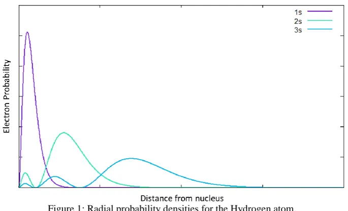
symmetrical, with smaller values as the distance from the nucleus increases. A single node (region where probabilities of finding electrons equal zero) is considered, occurring when this distance approaches infinity. This configuration changes depending on the principal quantum number, with a higher number of spherical nodes appearing as n increases, what can be seen by the radial probability densities of the orbitals 1s, 2s and 3s for the hydrogen atom plotted in Figure 1. Further, the variation of the azimuthal quantum number l will result in more complex forms for both orbitals and probability densities, as described in [22] and [24].
A hydrogen atom whose electron is in the lowest energy orbital, 1s, is said to be in its ground state. When the electron occupies any other orbital n ≥ 2, e.g. after receiving energy by the absorption of a photon, it moves to an excited state, name given to any quantum state with higher energy than the ground state. For the other atoms, the electron configuration of the ground state is the one in which the electrons occupy the orbitals of lowest energy available, obeying the Pauli Exclusion Principle and Hund’s rule [23]. The excitation condition results in an augmented average distance from the nucleus, and it usually tends to be transient (though there are exceptions where this condition can endure), with fugacious return of the atom to its ground state or to an excited state of lower energy by emitting a quantum of energy.
Figure 1: Radial probability densities for the Hydrogen atom.
IV.
OPTIMIZATION
THROUGH
AN
ATOMIC
EXCITATION
MODEL
The atomic theory exposed in the previous section served, somehow as a source of inspiration for the population-based neighborhood search metaheuristic proposed in this work. The adopted model consists of a mimicry of the modern atomic model, contemplating the description of the electronic distribution in its ground and excited states. Orbitals in this metaheuristic are, however, a simplified representation of what is found in the real atomic model, because they always have the form of a hypersphere with a single node, typical representation of the orbitals 1s, the most simple existent as reported in Section 3. Another simplification to be noticed in this model is that there is no analogy for the quantization of the energy of electrons, so they can assume continuous values according to the probability distribution adopted. A detailed description of the operation of the proposed algorithm, including these adaptations and other particularities of the project, is presented in the following paragraphs.The optimization process by this model starts with the definition of the required parameters for the operation of the algorithm. These include the number of atoms for the search (population size), the number of electrons for each atom, the search space (domain of the cost function including eventual restrictions) and the stopping criteria, which in this case are the maximum acceptable number of iterations and the minimum evolution between iterations for an atom.The atoms, in specified number, then have the initial positions of their nuclei established according to random coordinates, dictated by a continuous uniform distribution. For the electron clouds of these atoms, maximum and minimum investigation radii inside the search space are specified to warrant plausible limits for the position of the electrons. The value
r
min
0
.
01
n y y x xrmax max min max min
1
, (2)where n represents the population size and xmax, xmin, ymax, and ymin dictate the domain of the function to be
minimized. The procedure above described results in the minimum and maximum radii that can be used in a specific optimization problem, wherein at each iteration the individual search radii of each atom are recalculated within these limits. These individual radii (limits for the electron clouds) are calculated according to the set of values obtained for the cost function f (energy levels) at a particular iteration using Equation (3), also defined empirically:
f f f f r r r n n min max min 3 . 2 exp 1 max min . (3)This function tends to maintain the values of the investigation radii of the best atoms – those with the lowest values for the evaluation fn – closer to the minimum value rmin, at the same time keeping those of the worst
evaluated atoms closer to the maximum value (in fact, rmin rmax). In an analogy with the model that is source of inspiration for the algorithm, high values of the function to be minimized represent a more excited atomic state, meaning that the atom under consideration is at a higher energy level and, consequently, its electron cloud is distributed in a more dispersed form around its nucleus. In this way, these electrons will have greater freedom to explore, and can evaluate a wider area while pursuing a better path to the minimum of the cost function, that represents the position of lower energy and higher stability. In turn, the atoms that in a particular iteration have their nuclei located in more favorable positions, with lower values for the cost function, will be considered less excited. That less intense energy state will restrict the spread of the electron cloud, with the intention of proceeding with a more detailed search in the vicinity of these possible “sweet spots”. It is noteworthy that the ranking of the best atoms is updated at every iteration, thus an atom of low energy can move to a more excited state in the next step depending on the performance of another atom which may have found a better value for the cost function, for example.Within the limits for the scattering of the electron cloud of each atom at a given iteration, the electrons have their positions to evaluate the cost function defined stochastically. These positions are specified initially in the form of polar/spherical coordinates, wherein each point is represented by a radius (distance from the origin, in this case, the nucleus) and a number of angles equal to the problem’s dimensionality subtracted by one. Exemplifying with an easily comprehensible dimensionality, in a two variables function, x and y, the positions of the i electrons of each of the n atoms to evaluate the objective function f(x,y) will be scattered around the respective nuclei by specifying a distance from these i
n
r and an angle i
n
.The angles i n
are chosen as random values between 0 and 2π following a uniform distribution, while the distances from the nuclei in
r , while also random, follow the Rayleigh distribution, given by the equation (4):
2 22
2 exp |
z zz
g , (4)
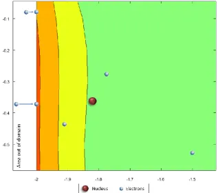
where it was adopted for the control parameter the value α = 1. This function was chosen because it corresponds to the distribution of the magnitude of a vector composed of independent random variables with Normal distribution, added to the fact that it resembles the real electronic distribution of the 1s orbitals, previously illustrated in Figure 1. Comparative tests performed with Normal and Uniform distributions support the choice of the Rayleigh distribution, after the latter resulted in slightly better results. The described way of calculating the electrons’ positions results in a radial symmetry for their distribution, as illustrated in the Figure 2 that simulates a “cloud” of electron density. From the values obtained in polar/spherical coordinates, the corresponding Cartesian coordinates, necessary for the function evaluation, are then calculated by the conversion equations (5) and (6):
i n i n i n rx cos
, (5)
i n i n in r
Figure 2: Electron density cloud simulated with Rayleigh distribution.
Being chosen by the described stochastic methods, the electrons’ positions must undergo a check of their contention to the search space. For this, each point generated, already converted to Cartesian coordinates, has its variables compared to their pre-defined limits. In case of a possible extrapolation in any of them, the electrons will be repositioned within the specified domain, according to the procedure shown in Figure 3.
Figure 3: Electrons repositioning inside function’s domain.
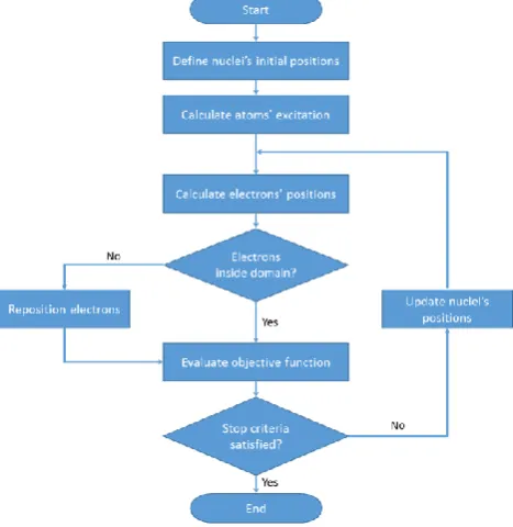
The sequence described in this section is illustrated in the flowchart of Figure 5.
Figure 4: Movement of an atom between iterations.
Figure 5: Flowchart representing the proposed algorithm.
V.
RESULTS
including monotonically decreasing functions and even multimodal functions with large numbers of local minima and traps. All the benchmark functions are continuous and unconstrained. This exposure to different challenges with various difficulty levels is important for allowing a good evaluation of the strengths and weaknesses of metaheuristics, and specially to test reliability, efficiency and validity of newly developed algorithms [25]. The selected functions are described in the sequence.
Benchmark 1: The six-hump camel back is a multimodal function defined by (7):
4 4
.3 1 . 2 4 , 2 2 2 2 2 1 2 1 4 1 2 1 2
1 x x x x x
x x x
x
f
(7)
This function has six local minima inside the considered domain, being two of them global: f(x1, x2) = -1.0316 at (x1, x2) = (-0.0898, 0.7126) and (0.0898, -0.7126) [25].
Benchmark 2: The second function tested here was a complex multimodal one, obtained from [12] and defined by (8):
x1,x2
x1 sin
4 x1
1.1 x2 sin
2 x2
,f (8)
with the global minimum f(x1, x2) = -18.5547 at (x1, x2) = (9.039,8.668). Benchmark 3: Rosenbrock’s Valley is a unimodal function calculated by (9):
100
1
.1 1 2 2 2 1
d k k kk x x
x x
f . (9)
This classical optimization problem is characterized by a long and narrow flat valley where the global minimum is found, with a difficult convergence [25] [26]. That minimum, corresponding to f(x) = 0 is obtainable for xk = 1, where d is the dimensionality of the problem and k = 1,…,d.
Benchmark 4: Rastrigin’s Function is a massively multimodal function mathematically represented by (10):
d k k k x x d x f 12 10 cos2
10 , (10)
with global minimum f(x) = 0 for xk = 0, where k = 1,…,d. A large number of local minima are regularly distributed around that point [26].
Benchmark 5: The simplest function used here is the one known as De Jong’s first function, consisting in an n -dimensional paraboloid defined by (11):
d k k x x f 1 2, (11)
what results in a convex and unimodal function with global minimum f(x) = 0 for xk = 0, where k = 1,…,d [26]. Benchmark 6: Easom’s function is a unimodal function defined by (12):
2
2 2 1 2 1 2
1,x cosx cosx exp x
x
x
f , (12)
with global minimum f(x) = -1 located at (x1, x2) = (π, π) [25]. This function is characterized by having its minimum inside a narrow pit surrounded by a large plateau.
Benchmark 7: Michalewicz’s function is a multimodal test function with values calculated by (13):
d k m k k x k x x f 1 2 2 sin sin
. (13)The parameter m controls the difficulty level of the problem, making the valleys more or less steep [26]. Here the value adopted is m = 20, and the global minimum f(x) = - 1.5971 is found at xk = 0 for the two-dimensional problem.
Benchmark 8: The last problem of this list is the Drop Wave Function, defined by (14):
2 5 . 0 12 cos 1 , 2 2 2 1 2 2 2 1 21
x x x x x x
f , (14)
(a) (b)
(c) (d)
(e)
(f)
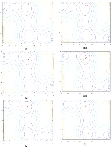
Figure 8: Comparison of performance of AE, GA and PSO for optimization of Function 2 with population n = 40.
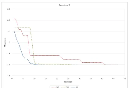
Figure 9: Comparison of performance of AE, GA and PSO for optimization of Function 7 with population n = 15.
Figure 10: Comparison of performance of AE, GA and PSO for optimization of Function 8 with population n = 50.
VI.
FINAL
REMARKS
analogy.
As a novel method, the Atomic Excitation model still have a large margin for improvements and addition of new features. Future work aiming further development includes more extensive testing, not only with theoretical benchmark functions but also with “real world” applications, followed by the correction of eventual weaknesses to be identified. Other possible points for improvement are the addition of flexibility on the selection of the probability density function (that defines the investigation area), a study on the performance gain (or loss) that could be brought by adding the capability of information exchange among the atoms, and a more extensive evaluation of the effects of changes in the control parameters on the performance of the optimization.
REFERENCES
[1] E. Elbeltagi, T. Hegazy, and D. Grierson, Comparison among five evolutionary-based optimization algorithms, Advanced Engineering Informatics, 19, 2005, 43-53.
[2] P. Hansen, and N. Mladenovic, Variable neighborhood search methods, in: C. A. Floudas, and P. M. Pardalos (Eds.), Encyclopedia of Optimization - 2nd Edition (New York, NY: Springer, 2009) 3975-3989.
[3] J.-S. Jang, C.-T. Sun, and E. Mizutani, Neuro-Fuzzy and Soft Computing: A Computational Approach to Learning and Machine Intelligence (Upper Saddle River, NJ: Prentice-Hall, 1997).
[4] C. Blum, and A. Roli, Metaheuristics in combinatorial optimization: overview and conceptual comparison, ACM Computing Surveys, 35(3), 2003, 268-308.
[5] D. E. Goldberg, Genetic algorithms in search, optimization and machine learning (Boston, MA: Addison-Wesley Longman Publishing Co., 1989).
[6] J. Kennedy, and R. Eberhart, Particle Swarm Optimization, Proc. IEEE International Conference on Neural Networks, Perth, Australia, 1995, 1942-1948.
[7] E. Rashedi, H. Nezamabadi-Pour, and S. Saryazdi, GSA: A Gravitational Search Algorithm, Information Sciences, 179(13), 2009, 2232-2248.
[8] R. A. Formato, Central force optimization: a new metaheuristic with applications in applied electromagnetics, Progress in Electromagnetics Research, 77, 2007, 425-491.
[9] O. K. Erol, and I. Eksin, A new optimization method: Big Bang–Big Crunch, Advances in Engineering Software, 37(2), 2006, 106-11.
[10] M. Dorigo, M. Birattari, and T. Stützle, Ant colony optimization, IEEE Computational Intelligence Magazine, 1(4), 2006, 28-39.
[11] D. Karaboga, and B. Basturk. A powerful and efficient algorithm for numerical function optimization: artificial bee colony (ABC) algorithm, Journal of Global Optimization, 39(3), 2007, 459-471.
[12] R. Rajabioun, Cuckoo optimization algorithm, Applied Soft Computing, 11, 2011, 5508-5518.
[13] K. S. Lee, and Z. W. Geem, A new meta-heuristic algorithm for continuous engineering optimization: harmony search theory and practice, Computer Methods in Applied Mechanics and Engineering, 194, 2005, 3902-3933. [14] A. Sadollah, A. Bahreininejad, H. Eskandar, and M. Hamdi, Mine blast algorithm: a new population based algorithm
for solving constrained engineering optimization problems, Applied Soft Computing, 13, 2013, 2592-2612.
[15] A. H. Kashan, League Championship Algorithm (LCA): An algorithm for global optimization inspired by sport championships, Applied Soft Computing, 16, 2014, 171-200.
[16] P. Hansen, and N. Mladenovic, Variable neighborhood search: principles and applications, European Journal of Operational Research, 130, 2001, 449-467.
[17] F. Z. Lebbah, and Y. Lebbah, VNS approach for solving a financial portfolio design problem, Electronic Notes in Discrete Mathematics, 47, 2015, 125-132.
[18] M. Khelifa, and D. Boughaci, A variable neighborhood search method for solving the traveling tournaments problem, Electronic Notes in Discrete Mathematics, 47, 2015, 157-164.
[19] J. Pereira, and M. Vilà, Variable neighborhood search heuristics for a test assembly design problem, Expert Systems with Applications, 42, 2015, 4805-4817.
[20] N. Dahmani, S. Krichen, and D. Ghazouani, A variable neighborhood descent approach for the two-dimensional bin packing problem, Electronic Notes in Discrete Mathematics, 47, 2015, 117-124.
[21] L. Pauling, General Chemistry -3rd Edition (Reprint) (Mineola, NY: Dover Publications Inc., 1988). [22] J. B. Russel, General Chemistry - 2nd Edition (New York, NY: McGraw-Hill, 1992).
[23] [23] T. L. Brown, H. E. Lemay, Jr., B. E. Bursten, and J. R. Burdge, Chemistry: The Central Science - 9th Edition (Upper Saddle River, NJ: Prentice-Hall, 2002).
[24] P. Atkins, and L. Jones, Chemical Principles: The Quest for Insight - 3rd Edition (New York, NY: W.H. Freeman and Co., 2005).
[25] M. Jamil, and X. S. Yang, A literature survey of benchmark functions for global optimization problems, Int. Journal of Mathematical Modelling and Numerical Optimization, 4(2), 2013, 150–194.