Modeling Complex System Using T-subnet based
Hierarchical Petri Nets
Zhijian Wang
Information Science School, Guangdong University of Business Studies, Guanzhou, China Email: [email protected]
Dingguo Wei
Information Science School, Guangdong University of Business Studies, Guanzhou, China Email: [email protected]
Abstract—Net compression technologies are widely researched to avoid the problem of state explosion. Current researches of transition refinement and subnet abstraction mainly paid attention to preserve different attributes during the transformation, usually led to very strict conditions for the subnet, so that the application of these technologies was limited. Aiming to provide the same service and interface after transformation as original module while less restricts are given, a kind of transition subnet is put forward to model complex manufacturing system. The concept “standardized interface” is presented; transition subnets are classified into different types, the idea of “normalized subnet” is presented; Engineering Subnet is defined and a live and normalized subnet with finite live loopbacks is proved to be an Engineering Subnet. Because of live loopbacks owned by Engineering Subnets, the same interface and service as the original module are reserved after the transformation between an Engineering Subnet and the corresponding transition, mean while fewer preconditions are required for the Engineering Subnet compared with current researches.
Index Terms—Petri nets, subnet, transition, interface, loopback
I. INTRODUCTION
Petri net was presented by Carl Adam Petri in 1962[1],
it is a modeling tool applicable to many systems, especially the discrete event dynamic systems [2]. Petri
nets provide users an intuitive system describing method because of their graphical describing ability; as a mathematical tool, a Petri net model can be described by linear algebraic equations reflecting the behavior of the system. Although Petri nets have become an important modeling method today and are widely used, modeling complex systems with common Petri nets directly brings the problem of state explosion, system modeling and analyzing become extremely difficult and sometimes impossible. To overcome this problem, modularization and hierarchy are effective methods supplementing each other; usually modularization forms the basis of hierarchy.
The primary measures to realize hierarchy in Petri nets are transition refinement and subnet abstraction. Transition refinement is used in top-down system
developing process, a subnet is designed to replace a transition and describe the function of that transition in detail; subnet abstraction is adopted in a bottom-up system developing process, a subnet is replaced by a transition so that the system model becomes more simple and understandable. Padberg presented a module concept for Petri nets, showed that the composition of modules preserves the property of safety[3]. Others researched the
refinement, synthesis and condense of subnets or modules in Petri nets[4,5]. Hierarchical Petri nets are widely
researched and applied, concepts such as reducible subnet, degree of subnet are defined by Lee[6].Hierarchical Petri
nets have been used to model complex systems [7-8].
Same interface and service are required during the substitution between a transition and a subnet, and keeping same interface is the basic requirement of modularization, same outputs are required when same inputs are provided. Current researches stressed preserving properties such as boundedness, liveness and reversibility in the process of substitution [3-5]. In
reference[8] a CO net for manufacturing systems was presented, CO net is a class of SISO Petri nets which is reversible, live, and keeps bounded; some refinement schemes were presented to apply Petri nets in complex flexible manufacturing systems [9,10].
For current researches there exists a conflict between the model equivalence and the modeling ability, usually too many strict restrictions are assigned to those subnets keeping good equivalence during the transformation [4-5,8-10], these restrictions limit the application of subnets
greatly. As an example, a subnet is required to return to its initial marking after the firing of a transition sequence from input transition tI to output transition tO in reference
[9], and the number of the tokens output by tO must equal
to that of what input by tI. Such requirements are very
difficult to be satisfied; in fact they are unnecessary in many occasions.
of transition subnets is presented to solve above problem, the subnet can run in succession and is called Engineering Subnet.
This paper is arranged in the following way: section 2 investigates the interface and surrounding environments of subnets; section 3 presents the idea to normalize subnets, section 4 discusses the test nets and loopbacks of subnets, in section 5 two types of markings are researched, section 6 defines the concept of Engineering Subnet and analyzes its attributes, at last a few conclusions are given in section 7.
II. SUBNET AND INTERFACE
Definition 1: Given a P/T net ,
if , ,
) ; , (PT F N = P
PS ⊆ TS ⊆T FS =((PS×TS)U(TS×PS)) and
is connected, then SN is the subnet of N.
F
I
) ; , (PS TS FS
SN=
Definition 1 originates in reference [12], but an extra condition is assigned that the subnet is required to be connected. This indicates the cohesion of a module; functions with no relationship are not allowed to be combined into the same module. Petri nets in this paper are connected P/T nets, namely the capacity function K is arbitrary but the weight function , in the rest of this paper they are called nets in short.
1 ≡
W
Every element or subnet interacts with its environment in the complete model.
Definition 2: Given a net (or subnet) ,
and :
) ; , (P T F N= T
P
x∈ U Y⊆PUT
(1)loc(x)={x}Ux*U*x is the local environment of x; (2)* { | ,( , ) };
F x y Y x y
Y = ∃ ∈ ∈
(3) * { | ,( , ) }; F y x Y x y
Y = ∃ ∈ ∈
(4) is the local environment of
Y;
Y Y Y Y
loc( )={ }U *U* (5)>Y=*Y−Y; (6)Y>=Y*−Y ;
(7)srd(Y)=>Y UY> is exterior environment of Y. Item (1), (2) and (3) originate in reference [12], item (4) is an extended definition by this paper.
The local environment loc(Y) is composed by two parts: Y and those outside Y. If the elements of Y form a subnet, the above two parts should be considered separately in actual application, so the concept “exterior environment” of Y is presented. For a subnet SN, the exterior environment can also be called “exterior interface”. is the exterior input transitions and places of SN (exterior input interface), is the output transitions and places of SN(exterior output interface), is the elements in N which interact with SN.
SN >
> SN
) (SN srd
Corresponding to exterior interface of subnets, inner interface or just interface in short, is defined in following definition 3.
Definition 3: Given a subnet , which
is the subnet of net
) ; , (PS TS FS
SN=
) ; , (PT F
N= :
(1) is the input
place interface set of SN;
)} (
|
{ ∈ ∧ * − ≠φ
= −
S S
P p p P p T
SNI
(2) is the output
place interface set of SN;
)} (
|
{ ∈ ∧ *− ≠φ
= +
S S
P p p P p T
SNI
(3) is the place interface set of SN;
+ −
= P P
P SN SN
SNI # U
(4) is the input
transition interface set of SN;
)} (
|
{ ∈ ∧* − ≠φ
= −
S S
T t t T t P
SNI
(5) is the output
transition interface set of SN;
)} (
|
{ ∈ ∧ *− ≠φ
= +
S S
T t t T t P
SNI
(6) is the transition interface
set of SN;
+ −
= T T
T SNI SNI
SNI # U
(7) is the input interface set of SN;
− −
− =
T
p SNI
SNI
SNI U
(8) is the output interface set of SN;
+ +
+ =
T
p SNI
SNI
SNI U
(9) # # # is the interface set of SN.
T
P SNI
SNI
SNI = U
Although the concept “border” was presented in reference [12], it was used to describe a set of transitions, places and corresponding arcs, it is more similar to the subnet in this paper, but maybe not connected. We consider “border” is more suitable to describe the physical border of a net.
Definition 4 : Given a subnet SN, if
, then SN is termed to be interface standardized.
SN SNI SN
SNI+) = >∧ ( −)=>
( * *
P2 P1
P3 t
...
(a) A non-standardized interface
P3 P1 t1 P0 t2 P2
...
(b) The standardized interface
Figure 1. An example of how to standardize a non-standardized interface
restrictions inside the subnet. From the standpoint of modularization, this means the input parameters of a lower layer module are provided by some upper layer ones, what inside a module is to realize its function and provides service for upper layer modules, the lower layer module doesn’t interfere the execution of the upper layer module. For the same reasons, a place in input interfaces works as a buffer of the module and accepts input variables; transitions inside the module decide how to use these variables, but they cannot influence the inputting. As to the input transition interfaces, the output transition or place interfaces, similar occasions come into existence. The interface in figure 1(a) is a non-standardized transition interface and it’s standardized in figure 1(b).
III. TRANSITION SUBNET
Definition 5: For a subnet , if
and , namely ,then
SN is called a transition subnet(T-subnet) and: ) ; , (PS TS FS
SN = φ
=
# P
SN SNT#≠φ
# #
T
SN SN =
(1)SN is a destination transition subnet( -subnet) if
( );
−
T
φ ≠
= −
T
SN
SN# SNT+=φ
(2)SN is a source transition subnet( -subnet) if
( );
+
T
φ ≠
= +
T
SN
SN# SNT−=φ
(3)SN is a normal transition subnet( -subnet) if
, .
#
T
φ ≠ +
T
SN SNT− ≠φ
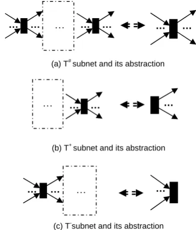
Transition subnets can be divided into several types according to their interfaces. Source subnets and destination subnets are named in allusion to their upper layer net models: if SN consumes tokens then it’s a destination subnet; if SN produces tokens then it’s a source subnet; if SN produces tokens after consuming tokens then it’s a normal subnet.
According to the number of inputs(SNI-) and outputs(SNI+) , subnets can be divided into different types as: ZI(Zero Input), SI(Single Input), MI(Multi Input), ZO(Zero Output), SO(Single Output) and MO (Multi Output). SISO -subnets are the most widely researched and applied T-subnets, what researched in reference [8] and [9] all belong to this type.
#
T
subnet abstraction is the process of replacing a T-subnet with a transition in order to simplify a complex Petri net model; it’s an important method to realize hierarchy in Petri nets. According to reference [12], abstraction is divided into simple abstraction and strict abstraction, from this point of view, what researched in this paper is (the extension of) simple abstraction, because strict abstraction doesn’t process subnet according to definition 1, it is in fact the fusion of transitions or places.
Above subnets and corresponding abstractions are listed in figure 2, what outside the dotted frame is the interface and what inside the dotted frame is the rest of the subnet.
Transition refinement is a reversed operation of subnet abstraction, which replaces a transition with a T-subnet. T-subnet abstraction is a bottom-up method and transition refinement is a top-down method.
Although the abstraction and refinement of net model operates reversely, they are not certainly mapped one to one. If a subnet SN is selected, the abstraction of SN is determined and no alternative exist. But for subnet refinement even the subnet SN and transition are determined, there exists different schemes for the mapping transformation between the arcs of and those of the subnet. According to the points of view in modularizing design, to define a module, only the inputs ( ), outputs ( ) and module function ( ) are required to be decided, the details of module realization is flexible.
N
t
N
t
N
t
* *
N
t tN
* → *
N
t
… … … … … … …
(a) T#subnet and its abstraction
…
… … …
(b) T+subnet and its abstraction
… …
… …
(c) T-subnet and its abstraction
Figure 2. Typical T-subnets and their abstraction
So if the preconditions and are satisfied, the structure of SN has different choices. According to firing rules of transitions, all inputs of a transition should be satisfied( : ), and all outputs will be obtained at the same time
( :
N
t SN=*
> *
N
t SN> =
N
t p∈*
∀ M(p)>0
* N
t p∈
∀ M(p)=M(p)+1), so the subnet SN should meet a condition, namely the execution of the subnet should consume one token from all places in and produce one token for every place in .
SN >
> SN
Intuitively there exist different subnet structures meeting above condition under the same surrounding environment. For a normal transition ( and
), the most intuitionistic method is to divide it into three parts as figure 2(a): the input part, the output part and the middle processing part. Guided by this idea, the concept of normalized subnet is presented in following definition 6.
N
t *tN ≠φ
φ ≠
* N
Definition 6: A subnet SN is termed as normalized subnet if: (1) SN is an interface standardized subnet; (2)
; (3) .
1 | | − ≤
SNI |SNI+|≤1
Intuitively all interface standardized SISO、SIZO、 ZISO subnets are normalized subnets, and are named normalized SISO subnets, normalized SIZO subnets and normalized ZISO subnets respectively, as for T-subnets, they are normalized -subnets, normalized -subnets and normalized -subnet. Although current researches focus on SISO subnets, SIZO subnets and ZISO subnets are widely used in actual system modeling.
#
T T−
+
T
Normalized T-subnets are not the only type of subnets meeting previous conditions, but they are the qualified subnets with the simplest interface and are easy to be defined explicitly. So we use normalized T-subnets as the standard subnet structures in the process of T-subnets based refinement and abstraction, other T-subnets can be transformed into normalized subnets if certain preconditions are met.
Subnet normalization helps to make a transition and the corresponding T-subnet looks similar - they own the same interface to their surrounding environment; but for subnet transformation, “looks similar” is not enough, “acts similarly” is required – the model should work almost the same way before and after the transformation (because of the difference of state spaces, the transformed model is impossible to be completely same as the original model). To make models act similarly, the behaviors of subnets must be studied carefully, so the test net is required.
IV. LOOPBACK OF SUBNET
To analyze a subnet, we usually transform the subnet into a live, bounded and token conservative test net, that’s the test net of subnet SN(labeled as SN ), this is
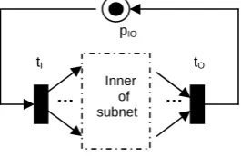
especially important if we want to analyze characteristics such as transition delay when time is introduced in the net model. Almost all current researches focus on SISO subnet, in a SISO subnet a close route can be setup by adding a test transition or place to connect the input and output elements together as figure 3.
Figure 3. Test net of T#-subnet
Since the subnets researched in this paper are not limited to SISO subnets, we have to discuss the test net in detail. For a normal transition subnet in figure 3, following two places are required in order to run independently: an input place working as the input of subnet from surrounding environment and an output place
working as the output of subnet to surrounding environment. In figure 3 we combine these two together as the place . Because a -subnet has no outside input, so the time to fire is decided by
I
p
O
p
IO
p T+
O
t SN itself;
similarly a -subnet outputs nothing to surrounding environment, the subnet finishes an execution if fires. Intuitively for a -subnet or a -subnet, in figure 3 can be deleted and that means its test nets is itself.
−
T
I
t +
T T− pIO
Definition 7: Given SN is the test net of subnet SN, if there exists a finite occurrence sequence
...
3 2 2 1 1tM t M
M
=
σ , tI and tO (if existed) occur in δ and occur only once, then τ=t1t2... is called a loopback of SN (or SN). If there exists no loopback τ' and
τ τ
θ< '< , then τ is a shortest loopback of SN (or SN). For the three types of subnets, their loopbacks are in the following forms of expressions separately:
(1)T#-subnet: { , , , } 2 1tI τ tO
τ
τ = ;
(2)T+-subnet: { , } 1tO
τ
τ= ;
(3)T--subnet: { , , } 2
1 τ
τ
τ = tI .
whereτ1,τ2={t1,t2...tn}are finite transition sequences
and , that means except
transitions in interface, the rest transitions inside the subnet can occur repetitively. The loopbacks set of SN is labeled as .
+ −− −
∈ S T T
n T SNI SNI
t t t1, 2...
) (SN Loop
The concept loopback is extended in definition 7, because for those ZI-subnet (T+-subnet) or ZO-subnet (T
-subnet), their test net is not close, so it’s impossible to connect their input and output so as to form a really close loopback. Also the subnet SN and its test net SN are not
distinguished when loopbacks are referred, namelyLoop(SN)=Loop(SN), because they contain the same transition sequences for a same loopback.
V. MARKING SETS OF SUBNET
A loopback make sure the subnet can execute once from input to output.
Definition 8: Given SM1⊆{M0S}UM0S[> (SM1 is
the subset of SN ’s initial marking and its reachable
markings), if ∀MS1∈SM1:∃MS2∈SM1 ,
) (SN Loop ∈
∃τ , MS2[τ >MS1, then is called the
first type marking set of
1
SM
SN , represented by LR1(SN). tI tO
pIO
… …
Inner of subnet
) ( 1SN
LR is the set of all markings reached by
loopbacks from the initial marking M0 . Intuitively S
) ( 1SN LR MS∈
∀ : MS(pIO)=1 . So places outside subnets ( ) keep its original marking after the firing of a loopback
IO
p
τ . SN and SN are not distinguished in such
A normalized T-subnet with loopbacks can execute like a transition at least once under the initial marking a reasonable assumption is that the system can return to its original marking after one of its execution, or return to a marking equivalent to the original marking, this means the model should own the attribute of repetitiveness. Furthermore, even repetitiveness is not necessary in some systems. A door lock with engineering key works correctly in all states before and after using the switching key, but it can not return to the original state any longer if the switching is used.
According to the idea of modularization design, a subnet should be able to run continuously, namely in the new marking reached after an execution, the subnet can still run correctly when outside inputs are ready.
Definition 9: Given , if
and
) ( 1 1 LR SN
SM ⊆
1 2 1
1 SM : M SM
MS ∈ ∃ S ∈
∀ ∃τ∈Loop(SN) ,
2
1[ S
S M
M τ> , then is a second type marking set of SN, represented by ;
1
SM
) ( 2SN
LR τ is called a live loopback.
A marking in may be “not live”, although it is reached by a loopback, it’s not sure that an other loopback can be founded under this state (it is not always a deadlock because there may still exist some transitions which can be fired); is a subset of , every marking in can reach itself or an other marking in by a live loopback, so the markings in are “live”, subnets in
can run continuously . ) ( 1SN LR
) ( 2SN
LR LR1(SN)
) ( 2SN LR
) ( 2 SN LR
) ( 2 SN LR )
( 2 SN LR
Only those loopbacks with finite length make sense to a subnet, a finite length loopback indicates a repetitive routine composed by steady transition sequence and every such repetitive steady transition sequence maps with a processing routine in a manufacturing system. A non live loopback can be used only once, after that maybe the system reaches a marking where no any loopback can be found any longer. “maybe” is used here because there may exist such loopbacks that can be executed only once, but after that the system reaches a live state where other loopbacks are existed. So a “not live” loopback does not mean “dead”, it just means a loopback can not be repeated.
A second type marking set of SN - can be divided into following different cases:
) ( 2SN LR
(1)LR2(SN)=ϕ.
In this case SN can not execute repeatedly and no live loopback exist. Such case is not researched any longer in this paper.
(2) LR2(SN)={M0S} , ∃τ∈Loop(SN) ,
S
S M
M0 [τ> 0 .
This case is the presupposition of the research in reference [9] that SN returns to its initial marking after the firing of a loopback.
(3)∃MS1∈M0S[>,LR2(SN)={MS1},∃τ∈Loop(SN) ,MS1[τ>MS1.
This is the extension of case (2), the system enters a circular executing state in marking . Suppose
,this can be a initialing process in advance in a real manufacturing system, after this the system begins a fixed operating routine
1 S
M
1 3 2 2 1
1 ...
0StMSkt MSk t MS
M
) ,... , (t1 t2 tn
τ to produce repeatedly. In case (2) we can regard that the system is initialized in the same way by , so can be regarded as part of the processing routine. Of course n=0 is possible, that means initialization is unnecessary in this system. In case (3) the system is required to be initialized only once (in certain time period).
) ,... ,
(t1 t2 tn (t1,t2,...tn)
(4) MS1,MS2,MS3...∈LR2(SN) and ...
3 2
1 S S
S M M
M ≤ ≤ , LR2(SN) is an infinite set.
This is the case close to a recurrence system where a marking is covered by the markings reached from it. This case is not always to be a recurrence system, because the subnet is not always to be a live one since there may exist not live transitions. Intuitively unbounded places may exist in this case.
(5) , and each form a marking
set as case (3) or case (4); or forms similar system by the combination of several loopbacks.
U
SMiSN
LR2( )= SMi
This is the extension of case (3) or case (4).
(6) and the conditions in case (5) are not satisfied.
2 | ) ( 2 |LR SN ≥
In this case the markings in can be reached each other by loopbacks, that the system is revertible. In a real system usually is a finite set, so the live loopbacks in the system is finite.
) ( 2SN LR
) ( 2SN LR
VI. ENGINEERING SUBNET
According to the analysis above, the subnet which can be executed continuously is defined as following.
Definition 10: A normalized T-subnet SN is called an Engineering Subnet if:
(1)∀MS1∈M0S[>, if then is included in a loopback
> 1 1[t
MS t1
τ ;
(2)Loop(SN)=LP1ULP2, where is a non-empty,
finite set of live loopbacks, is a finite set of loopbacks; and
1
LP
2
LP
2
LP
∈
∀τ : M0S[τ >MS1
) ( 2
1 LR SN
MS ∈
∧ , or ∃τ11,τ12...τ21,τ22...∈LP2 ,
1 22
21 12
11, ... , , ...
[
0S MS
M τ τ ττ τ > ∧MS1∈LR2(SN).
corresponds to a initialing process, so the subnet will not trap into a “not live” marking.
Next we will analyze the relationship between subnet’s liveness and its continuously executing ability. When we say a subnet SN is live we means its test net SN is live,
because a subnet is not a complete net, whether its transitions can fire or not relies on its surrounding environment, so is not only decided by itself. If surrounding conditions is not satisfied, the subnet can not execute, but its test net is a complete net which can exist and execute independently.
Corollary 1: A live and normalized subnet owns and only owns live loopbacks.
Proof:
(1) Given a normalized -subnet SN, since SN is live, there must exist a transition sequence
+
T
1
τ ( is not included in
O
t
1
τ ,τ1 may be empty), where M0S[τ1>MS1,
, then
2
1[O S
S t M
M > τ=(τ1,tO) forms a loopback and
, so SN owns loopbacks. , since SN is live, there must exist )
( 1
2 LR SN
MS ∈
) ( 1
1 LR SN
MS ∈ ∀
1
τ (tO is not included in τ1 ), where MS1[τ1>MS2 ,
3
2[ O S
S M
M τ > , let τ=(τ1,tO), then τ forms a loopback;
above process can be repeated for MS3, so τ is live, and . In this way we can prove all elements in belong to , and every loopback of SN is live.
) ( 2
1 LR SN
MS ∈
) ( 1SN
LR LR2(SN)
(2)Similarly to above process, we can prove a normalized -subnet SN owns loopbacks and every loopback of SN is live.
−
T
(3)Given a normalized -subnet, since SN is live, there must exist transition sequences
#
T
1
τ and τ2( and are not included in
I
t
O
t τ1 and τ2,τ1 and τ2 may be
empty), where M0S[τ1>MS1 , MS1[tI >MS2 ,
3 2
2[ S
S M
M τ > (since in tI SN can not be fired again
before tO is fired, so the transition sequence τ2 contains
no tI must be existed), MS3[tO>MS4 , then )
, , , (τ1tI τ2 tO
τ = forms a loopback, then M0S[τ>MS4,
and so SN owns loopback; , since SN is live, there must exist transition sequences
) ( 1
1 LR SN
MS ∈
∀
1
τ and
2
τ (tI and tO are not included in τ1 and τ2), where
2 1
1[ S
S M
M τ > , MS2[τI >MS3 , MS3[τ2>MS4 ,
5
4[ O S
S M
M τ > , let τ =(τ1,tI,τ2,tO), then τ forms a
loopback; above process can be repeated for MS5, so τ is live and ; In this way we can prove all elements in belong to , and every loopback of SN is live.
) ( 2
1 LR SN
MS ∈
) ( 1SN
LR LR2(SN)
With (1), (2) and (3) together, corollary 1 is proved. According the proof process of above case (3) in corollary 1, and the properties of normalized -subnet, following corollary 2 is obtained.
#
T
Corollary 2: In a live and normalized -subnet SN, the firing of is the sufficient and necessary condition to fire .
#
T
I
t
O
t
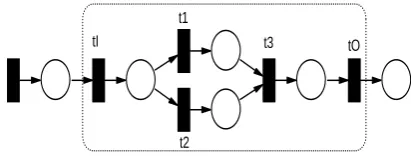
So a subnet SN is not certainly to be a live one even every transition in SN is live when SN is treated as a part of the complete net model. t3 in figure 4 can be live if it
is a transition in a complete model, but we can find the subnet is not live by constructing its test net, the reason here is because the subnet doesn’t satisfy the requirements in corollary 2.
tI
t1
t2
t3 tO
Figure 4. A not live subnet
Corollary 3: A live and normalized T-subnet with finite loopbacks is an Engineering Subnet.
Proof:
(1) We first prove if an arbitrary transition is fired, then is contained in a loopback.
1
t
1
t
> ∈
∀MS1 M0S[ , suppose M0S[τ1>MS1 ( τ1 is a
transition sequence and may be empty). If , since SN is live, so:
2 1
1[ S
S t M
M >
a) For transition in a -subnet SN, there must exists transition sequence
O
t T+
2
τ (τ2 contains no tO), so that
3 2
2[ S
S M
M τ > and MS3[tO>; if is not contained in tO
1
τ , according the specialties of normalized -subnet,
+
T )
, , , (τ1t1τ2 tO
τ = forms a loopback; if is contained in
O
t
1
τ , let τ1=(τ11,tO,τ12, tO...τ1n−1,tO,τ1n),
then τ =(τ1n,t1,τ2,tO) forms a loopback.
b) For transition in a -subnet SN, similarly to the process in a), we can prove if an arbitrary transition is fired, is included in a loopback
I
t T−
1
t
1
t τ ,
c) If SN is a -subnet, we have to discuss it in different cases.
#
T
If the firing of has nothing to do with and (t1 tI tO τ1
is unnecessary to contains and ), then: if and are not contained in
I
t tO tI tO
1
τ , select a arbitrary loopback τ2,
then τ =(τ1,t1,τ2) forms a loopback and is contained in
1
t
τ ; if and tI tO are included in τ1, let ''τ1 represents
the transition sequence from the beginning to the last in
O
t
1
τ (which is a loopback), 'τ1 represents the transition
sequence by take out ''τ1 from τ1, select an arbitrary
) , ,' (τ1 1τ2
τ = t forms a loopback and is contained in t1 τ .
If the firing is associated with and , then at least one of and is included in
1
t tI tO
I
t tO τ1, intuitively in τ1
the number of will not be greater than that of (conclusion 1), because according to corollary 2, only one firing of is required to fire once; If and are required to fire many times so as to firing , namely
and occurred in
O
t
I
t
I
t tO tI tO
1
t
I
t tO τ1 many times, since SN is live,
so the firing of every pair of and has nothing to do with other and , so the transition sequence of
I
t tO
I
t tO τ1
can be adjusted as ,
, , , (
' 11 12 1 τ tI τ tO
τ = τ13,tI,τ14,tO...τ1n−2,tI,τ1n−1,tO,τ1n+1, ...)
, , 1n 2 I
I t
t τ + , suppose after the firing of the last the
reached marking is , since
O
t '
1 S
M (τ11,tI,τ12,tO) , )
, , ,
(τ13 tI τ14 tO … all form loopback separately, so
, take out the loopbacks from '
1 S
M ∈LR1(SN) τ1', let
...) , , , (
'' 1 1 1 2 1 = τn+ tI τn+ tI
τ , then MS1'[τ ''>MS1, and τ1''
contains no , it’s composed by some and other transitions(conclusion 2), to simplify the expressions,
O
t tI
1
τ is represented by τ1'' in the rest of the proof; if occurs in
I
t
1
τ m times and , since SN is live, then all and are live, so is at most the precondition of firing one , it means for all corresponding to the rest ( ) , their firing don’t require to be fired in advance, so in the , we can find transitions to form loopbacks before the firing of , similar to the simplifying method used in the proof of conclusion 2, we change
1 >
m tI
O
t t1
O
t tO
1 −
m tI t1
1 S
M 1
−
m t1
1
τ into τ1=(τL,τ11,tI,τ12) , where τL is the
loopbacks composed by , and corresponding transitions, suppose
1 −
m tI tO
2
1[ L S
S M
M τ > , then
, let
2 S
M ∈LR1(SN) τ1'=(τ11,tI,τ12) then MS2[τ'>MS3,
so MS3[t1> ( is live in t1 SN , and loopbacks of SN can
only fire in sequence, so the firing of m−1 in advance will not affect ), suppose , because is reached from a first type marking by firing once, so there must exists
O
t
1
t MS3[t1>MS4
4 S
M MS2
I
t τ2( and are
not included), so that
I
t tO
5 2
4[ S
S M
M τ > , MS5[tO> ,let
) , , ,' (τ1 t1τ2 tO
τ = , then τ forms a loopback containing . t1
So in case a), b) and c), if an arbitrary transition is fired, is included in a loopback
1
t
1
t τ , the restrict (1) in
definition 10 is satisfied.
(2)The second restrict in definition is ,according to preconditions, the number of loopbacks is finite, take corollary 1 into account, so is a non-empty, finite set of live loopbacks,
2 1
)
(SN LP LP
Loop = U
1
LP φ
= 2
LP .
With the proof of (1) and (2) together, Corollary 3 is proved.
t2
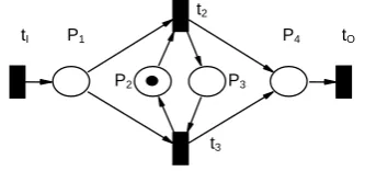
Figure 5. An example manufacturing system
An example of engineering subnet is the manufacturing system in figure 5. There exist two devices with completely same functions and performances, they can transform a rough part (the token in p1) into a finished product (the token in p4), where:
(1) tI is the inputting transition to obtain a rough part
into place p1;
(2) p2,p3 are the tokens to operate these two devices;
(3) t2 and t3 represent the processing of the part p1 by
two same machines respectively.
(4) p4 is the buffer of the finished products;
(5) tO indicates the delivery of finished products.
This example is ordinary in real systems such as a dual server system. The model doesn’t satisfy the requirements in reference[9], because the two markings M1=[x,1,0,y] and M2=[x,0,1,y] is different, but since the
two machines work in the way, they make no difference to outside environment, the system always runs correctly when outside conditions are satisfied.
VII. CONCLUSION
Engineering Subnets aim to satisfy the requirements of hierarchical and modular modeling in a complex system but relatively relaxed restricts will be assigned. When Engineering Subnets are used to transform a model, the primary precondition is the attributes they owned, especially the existence of live loopbacks, the requirement of existing live loopbacks is relatively loose than that of current researches. The abstraction operation is to simplify the original model, in this case attributes of the net are relatively easy to be reserved; for system refinement, attributes of the net can be reserved under certain preconditions. Normalization of subnets solve the problem of making a subnet and the transition “look similarly”, namely their interfaces to surrounding environments are the same; “live loopback” solves the problem of how to make a subnet and a transition “behave similarly”.
If a subnet is required to be live, then every transition in the sub system should be live, but in an actual application system this is usually unnecessary. Maybe something is wrong in a module and results that some of its minor functions can not be executed successfully (corresponding transitions is not live ), but the main functions still keep available, to surrounding environment the modular is still effective in such occasion. The precondition of Engineering Subnets is that the principal parts of a subnet are normal and the subnet will not
tI
t3 P1
P2 P3
cumber the rest of the system, namely there still exists live loopbacks in its test net, so the modular can input and output normally.
ACKNOWLEDGMENT
This paper is based on “A Class of Petri Nets for Modular and Hierarchical System Modeling”, which is appeared in proceedings of ICYCS2008.
Project supported by the Natural Science Foundation of Guangdong Province (Grant No. 8451032001001610 ), Natural Science Foundation of Guangdong Province (Grant No. 0630970 ).
REFERENCES
[1] T. Murata, “Petri Nets: Properties, Analysis and
Applications”, Proceedings of the IEEE, 1989, vol. 77(4),
pp. 541-580.
[2] J. H. Noguera, E. F. Watson, “Analyzing Throughput and Capacity of Multiproduct Batch Processes”, Journal of Manufacturing Systems ,2004, vol. 23(3) , pp. 215-228.
[3] J. Padberg, “Safety Properties in Petri Net Modules”,
Journal of Integrated Design & Process Science, 2004,
vol. 8(4), pp. 65 - 78.
[4] H. Huang, T. Y. Cheung, W. M. Mak, “Structure and behavior preservation by Petri-net-based refinements in system design”, Theoretical Computer Science, 2004, vol. 328(3), pp.245−269.
[5] V. Khomenko, K. Alex, K. Maciej , “Merged processes: a new condensed representation of Petri net behaviour”,
Acta Informatica, 2006, vol.43(5), pp.307-330.
[6] K. H. Lee, J. Fabrel, “Hierarchical reduction method for analysis and decomposition of Petri Nets”, IEEE TRANS. SYST. MAN. CYBER, 1985, SMC-15(2), pp. 272-280.
[7] M. Tittus, B. Lennartson, “Hierarchical supervisory
control for batch processes”, IEEE Trans. on Control Systems Technology, 1999, vol.7 (5), pp. 542-554. [8] J. M. Proth, L. Wang, X. Xie, “A Class of Petri Nets for
Manufacturing System Integration”, IEEE Transactions on Robotics and Automation, 1997, vol. 13(3), pp.317-326.
[9] C. L. XIA, L. JIAO, W. M. LU, “Petri Net Refinement
and Its Application in System Design”, Journal of
Software, 2006, vol.17(1), pp.11-19 (in Chinese).
[10] J. Padberg, M. Gajewsky, C. Ermel, “Rule-Based
refinement of high-level nets preserving safety properties”,
Science of Computer Programming, 2001, vol.40,
pp.97-118.
[11] C. Y. Yuan, Petri Nets Theory and Application, Beijing:
Publishing House of Electronic Industry,2005.
[12] C. Girault, R. Valk, Petri Nets for Systems Engineering: A Guide to Modeling, Verification, and Applications, Berlin:
Springer-Verlag, 2002.
Zhijian Wang was born in Changsha, Hunan Province, China in 1970. He obtained his Ph.D. degree in Control Theory and Control Engineering from Central South University in 2007 in China.
He is presently an associate professor of Computer Science in Information Science School, Guangdong University of Business Studies, Guangzhou, China. He is also the senior member of China Computer Federation. His current research interests include Petri nets, software engineering, and Computer Integrated Manufacturing Systems.
Dingguo Wei was born in Hunan Province, China in 1964. He obtained his Ph.D. degree in Computer Software and Theory from Fudan University in 2003 in China.