The Nonlinear Variable Selection and Its Realtime Detection of Lead-acid Battery Capacity

(1)

The Nonlinear Variable Selection and Its

Real-time Detection of Lead-acid Battery Capacity

Yingying Su1,2

1_{College of Automation, Chongqing University, Chongqing, 400044}

Email:[email protected]

Xinghua Liu2_{, Shan Liang}1,*_{, Jingzhe Lee}2_{, Lizhong Yao}2_{and Kesheng Yan}3

2_{School of Electric and Information Engineering, Chongqing University of Science and Technology, Chongqing,}

401331

3_{School of Mathematics and Statistics, Chongqing University of Technology, Chongqing, 400054}

Email: [email protected]

Abstract—Real-time detection of lead-acid battery capacity

is hard for not having the suitable instrument. The soft sensing method is considered. It is studied on the basis of variable selection, the confirming of structure and parameters for the predicted model. The importance of each related nonlinear secondary variable is computed and sorted with RReliefF method. After that, the secondary variable sets are selected in turn. Soft sensing model with neural network is finally confirmed by cross-validation method. Simulation results show that the established model is effective with mean square error is 0.0011 for the testing data. It provides one way of simplifying the real-time detection of battery capacity.

Index Terms—variable selection, real-time, detection,

lead-acid battery, capacity

I. INTRODUCTION

Constant exile electrical method is the main way of battery capacity detection with the problems of long operation time, large workload, amounts of power-consuming, difficulty to conduct and high cost [1-5]. To solve the above problems, the manufacturers of the capacity find that lead-acid battery capacity of discharging termination voltage can be indirectly reacted after testing the size of the battery capacity through a large number of testing data and expert experience. Inspired by this, the discharge capacity of the battery is established through the variable selection during all the possible variables in order to achieve the purpose of indirectly sensing the battery capacity [6-8]. The model is designed to make the battery production cycle becoming shorter and more applicability, to achieve energy conservation and consumption reduction, to improve the product factory qualified rate, intelligent, finally to realize the battery cost reduced, to adapt to the modern industrial development.

Soft sensing based on process mechanism analysis

needs users to understand the process clearly, in order to make soft instrument in good performance, and easy to implement applications. Therefore, it is difficult to obtain the sensing of battery [9-12]. The method based on state estimation requires accurate object, and usually only gets a simplified mathematical model of the process, whose white noise is far away from our expectation. This method is mainly used to estimate and track the location of the target of all kinds of sports, speed and trajectory in military field or robot [13-16]. The soft sensing method based on regression analysis is classic, simple and practical, whose application scope is quite wide. The sensing model is sensitive to errors by analyzing a lot of samples (data) [17-20].

By the analysis of the lead-acid battery and its production process, it shows that only parts of the secondary variables of its characteristics and production process of lead-acid battery can be measured, while its production process is highly nonlinear complex systems, which is unable to control [21-24]. Taking a power system of lead acid battery production technology in Chongqing Valve Control Limited Company for example, the soft sensing of battery capacity are solved first for the variable selection on the basis of the formula, craft obtained long-term from the company accumulation, and the rich real-time data of battery performance. With data mining method, the soft sensing is then worked out with only measure a little of battery performance parameters instead of all, which provides theoretical feasibility of omitting the battery discharge capacity in the process of production inspection, achieving the goals to reduce energy consumption and cost savings.

II. FORMATION OF LEAD-ACID BATTERY

Lead-acid battery is mainly composed of battery slot, battery cover, positive/negative plate, dilute sulphuric acid electrolyte, septum, and accessory. The chemical reaction called Formation is the most important part, which determines the capacity. It has two types: (1) Counter Electrode Formation; (2) Battery Formation. Normally, the first type is easily controlled in the producing course, whereas it may result in environment

Manuscript received April 1, 2013; revised June 1, 2013; accepted July 1, 2013.

(2)

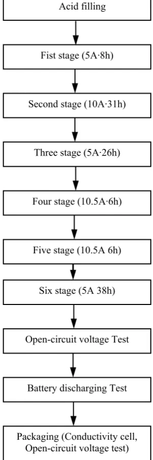
pollutions. The cost of the second type is lower, and its shortcoming is difficultly controlled and highly required to the quality of counter electrode. In that way, the manufacturing technique is usually chosen as the second one for most departments, where its Formation course is shown in Figure1.

Figure 1. The course of Battery Formation

III. RRELIEFFALGORITHM

With feature selection of regression algorithm RReliefF [25], the importance of each original secondary variable is calculated, respectively, according to the following steps:

(1) Select the sample D_ifrom sample set, and choose

the k samples nearest to Di from the rest of the m−1

samples and then repeat the course for 1≤ ≤i m;

(2) Calculate weight set ndC of sample Di under the

condition of its dominant variable value P₀. The equation

(1) is as follows:

k P P

P P n

k

i

i dC

1

min max

1 0

• −

− + =

∑

=

(1)

0

P stands for the dominant variable P value of the

sample Di, Pi （

1 ≤ ≤

i

k

）is the dominant variable

value of the sample i, Pmax and Pmin is the maximum

and the minimum of m samples;

(3) Calculation weight set n_dA[ ]A of the sample Di

under the condition of original secondary variable A. The equation (2) is as follows:

[ ]

k A A

A A A

n

k

i

dA

1

min max 1

0

• −

− +

=

∑

=

(2)

0

A stands for the original secondary variable A value of the sample D_i, A_i(1≤ ≤i k）is the original secondary

variable value of the sample i , Amax and Amin is the

maximum and the minimum of m samples;

(4) Calculate weight set n_dC_&_dA

[ ]

A of the sample D_i

under the condition of the dominant variable P₀ and the

original secondary variable A. The equation (3) is as follows:

[ ]

∑

=

⎟⎟

⎠

⎞

⎜⎜

⎝

⎛

−

• −

−

=

k

i

i i

dA dC

A

P

k

A

n

1 max min

0 min max

0 &

1

(3) (5) Repeat the four steps m−1 times, each time different samples are selected, obtaining ndC , n_dA

[ ]

A ,

[ ]

& dC dA

n A ;

(6) CalculateN_dC ,NdA

[ ]

A , including NdC&dA

[ ]

A in turn:

Where dC

N is the sum of

n

dC among all the m

ones,

[ ]

dA

N A is the sum of ndA

[ ]

A among all the m ones;N_dC_&_dA

[ ]

A is the sum of n_dC_&_dA

[ ]

A among all the

m ones;

(7) Use the following type to calculate weight value [ ]

W A of the original secondary variable A, the equation (4) is as follows:

[ ]

(

)

(

)

&

& dC dA dC

dA dC dA dC

W A N A N

N A N A m N

= −

− −

：

(4)

All weights are calculated according to the original secondary variables.

IV.MODELING OF SYSTEMS BASED ON NN

Acid filling

Fist stage (5A·8h)

Second stage (10A·31h)

Three stage (5A·26h)

Four stage (10.5A·6h)

Five stage (10.5A 6h)

Six stage (5A 38h)

Open-circuit voltage Test

Battery discharging Test

(3)

NN can emulate the physical structure as well as the memory function of mankind brain. It has been testified as a universal function approximator on mathematics, and can approximate every nonlinear function in L2 _{norm. In}

this way, it is an effectively method in solving the function modeling problems, where the characteristic pattern is implicit. In hundreds of NN types, multi-layer feedforward NN is one of the widely adopted models.

Usually, multi-layer feedforward NN adopts Back Propagation (BP) as learning algorithm. Its learning procedure is as following:

Confirm the topological structure and the learning parameters of NN:

(1) Initialize the weight and threshold values of NN; (2) Obtain the training data: input vector Xp and target

vector Y_p;

(3) Compute the state of hidden layer neurons and the actual output of NN, (Sigmoid function is supposed as the active function); )] ( exp[ 1 1 ) (

∑

− − + = − = k j kj k j kj k pk O W O W f O

θ

(5)

(4) Compute the value of error energy function;

∑

= − = n k pk pk

p Y O

E 1 2 ) ( 2 1 (6)

(5) Compute the training error of current NN: output-layer:

) )(

1

( _pk _pk _pk

pk

pk =O −O Y −O

δ

(7)

hidden layer:

∑

− = k kj pk pj pj

pj O O

δ

W

δ

(1 ) (8)

(6) Adjust weight and threshold values:

)) 1 ( ) ( ( ) ( ) 1 ( − − + + = + n W n W O n W n W ji ji pj pj ji ji

α

ηδ

(9) )) 1 ( ) ( ( ) ( ) 1 ( − − + + = + n n n n j j pj j j

θ

α

ηδ

θ

(10)

Turn to step (5), or stop at the stopping epoch, or the error energy function has been satisfied.

V. LEAD-ACID BATTERY PRODUCTION DATA AND

STREAMLINE SOFT SENSING

This paper studies lead-acid battery TD100F4 in a ChongQing Company as the research object. More than 300 groups battery data and 700 function test data are selected since April 8, 2012 to April 23, 2012 shown in TABLE I, TABLE II. Due to the restricted by technical conditions, eliminate some wrong and incomplete data, remaining the rest battery data 200 groups, function test data of more than 700 groups. With RReliefF variable selection method, three secondary variables data set are determined depending on the interpretation ability of each variable, and BP neural network is used to established the soft sensing of the battery capacity model with the same

method as front to sort out secondary variables in turn, in order to join the data in neural network modeling.

Taking the capacity of lead-acid battery production in the process of discharging termination voltage for example, the battery goes through six stages to charge and discharge capacity. Capacity and discharge detection rate involves in measuring 10 hours discharging termination voltage.

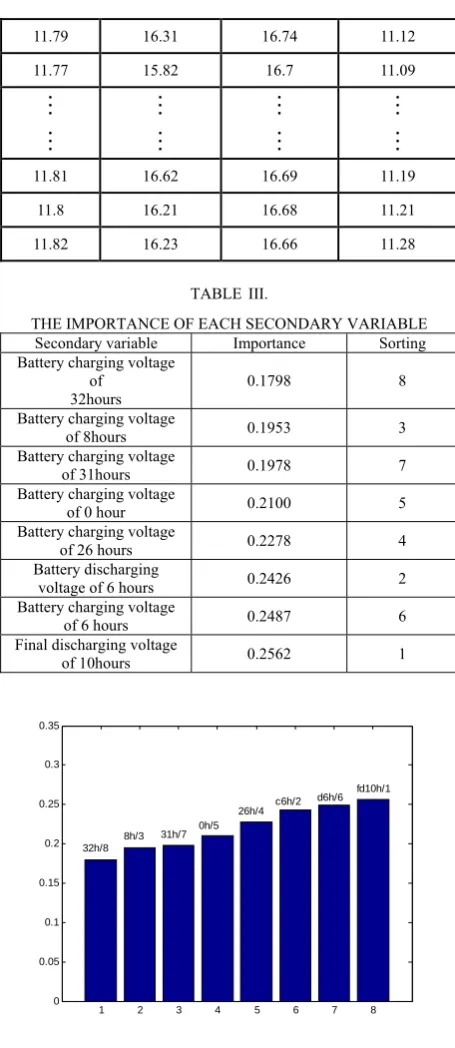
The original secondary variables are selected as battery charging voltage of 32 hours battery, battery charging voltage of 31 hours, battery charging voltage of 26 hours, battery charging voltage of 8 hours, battery charging voltage of 6 hours (c6h), battery discharge voltage of 6 hours (d6h), battery discharge voltage of 0 hour, and final discharging voltage of 10hours. The number of sample set

is 172. After that, the importance of eight original secondary variables is obtained with RReliefF method shown in TABLE III and Figure2.

TABLE I.

THE ORIGINAL SAMPLES Battery charging voltage of 8hours Battery charging voltage of 31hours Battery charging voltage of 26hours Battery discharging voltage of 0 hour

12.33 16.21 16.44 12.55

12.24 16.31 16.58 12.52

12.11 16.36 16.53 12.89

12.33 16.18 16.46 13.11

12.32 16.23 16.42 13.11

12.3 16.23 16.52 13.1

12.32 16.24 16.52 13.08

12.25 16.12 16.5 13.06

#

12.08 16.28 16.46 12.53

12.25 16.2 16.42 12.55

12.17 16.22 16.41 12.56

TABLE II.

THE CONTINUED SAMPLES Battery

charging voltage of 6

hours Battery charging voltage of 6hours Battery charging voltage of 32hours Final discharging voltage of 10hours 11.79 16.59 16.71 11.25

11.75 16.48 16.76 11.28

11.81 16.52 16.77 11.34

11.74 16.11 16.69 11.16

11.78 16.34 16.72 11.16

(4)

11.79 16.31 16.74 11.12

11.77 15.82 16.7 11.09

#

11.81 16.62 16.69 11.19

11.8 16.21 16.68 11.21

11.82 16.23 16.66 11.28

TABLE III.

THE IMPORTANCE OF EACH SECONDARY VARIABLE

Secondary variable Importance Sorting

Battery charging voltage of

32hours

0.1798 8

Battery charging voltage

of 8hours 0.1953 3

of 31hours 0.1978 7

of 0 hour 0.2100 5

of 26 hours 0.2278 4

Battery discharging

voltage of 6 hours 0.2426 2

of 6 hours 0.2487 6

Final discharging voltage

of 10hours 0.2562 1

1 2 3 4 5 6 7 8

0 0.05 0.1 0.15 0.2 0.25 0.3 0.35

32h/8

8h/3 31h/7 0h/5

26h/4 c6h/2

d6h/6 fd10h/1

Figure 2. The contribution sorting of each variable

(variable/ serial number)

According to this data set, in the learning process of BP neural network, each group is randomly selected with 130 samples as training data, 42 samples as the test data, which are all trained 10 times.

A. The Online Detection with all the Eight Secondary Variables

Taking the accuracy of built model with 8 secondary variables as the example in Figure 3, the outputs accuracy of Neural Network are compared with training data, relative error with different models. The number of hidden layer nodes in BP neural network is determined as

15 by interaction validation method. network training and testing prediction are shown in Figure 4 and Figure 5.

-250 -200 -150 -100 -50 0 50 100 150 200 250 -200

-150 -100 -50 0 50 100 150 200

32h 8h 31h 0h 26h c6h d6h fd10h

battery capacity

Figure 3. The NN detection of battery capacity with all secondary

variables

0 20 40 60 80 100 120 140 11

11.05 11.1 11.15 11.2 11.25 11.3 11.35

Samples

O

ut

put

Training Predicted Output by BPNN

Training Predicted Output Training Expected Output

(a) The output of NN compared with the real value

0 20 40 60 80 100 120 140 -1.5

-1 -0.5 0 0.5

1 Training Relative Error by BPNN

R

e

la

ti

v

e

E

rr

o

r(

%

)

Samples

(b) The error between the output of NN and real value

Figure 4. The outputs and the relative errors of the 130 training

(5)

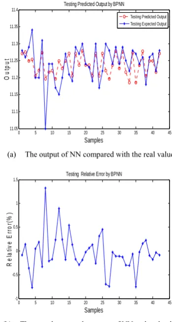
0 5 10 15 20 25 30 35 40 45 11

11.05 11.1 11.15 11.2 11.25 11.3 11.35

Samples

O

ut

put

Testing Predicted Output by BPNN

Testing Predicted Output Testing Expected Output

0 5 10 15 20 25 30 35 40 45 -1.2

-1 -0.8 -0.6 -0.4 -0.2 0 0.2 0.4 0.6 0.8

Testing Relative Error by BPNN

Re

la

ti

v

e

E

rr

o

r(

%

)

Samples

Figure 5. The outputs and the relative errors of the 42 testing samples

under the 8-1 model

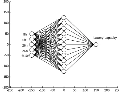
B. The Online Detection with the Selected Former Five Secondary Variables

On the basis, the original secondary variables are selected as the first five important variables where the number of hidden layer nodes in BP neural network is 11 determining by interaction validation method in Figure6. The final network training and testing prediction are shown in Figure 7 and Figure 8.

-250 -200 -150 -100 -50 0 50 100 150 200 250

-200 -150 -100 -50 0 50 100 150 200

8h 0h 26h c6h fd10h

battery capacity

Figure 6. The NN detection of battery capacity with the former five

secondary variables

0 20 40 60 80 100 120 140 11

11.05 11.1 11.15 11.2 11.25 11.3 11.35 11.4 11.45

Samples

Ou

tp

u

t

0 20 40 60 80 100 120 140 -1.5

-1 -0.5 0 0.5 1 1.5 2 2.5

Training Relative Error by BPNN

R

e

la

ti

v

e

E

rr

o

r(

%

)

Samples

samples under the 5-1 model

0 5 10 15 20 25 30 35 40 45 11

11.05 11.1 11.15 11.2 11.25 11.3 11.35

Samples

O

ut

put

0 5 10 15 20 25 30 35 40 45 -1.2

-1 -0.8 -0.6 -0.4 -0.2 0 0.2 0.4 0.6

R

e

la

ti

v

e

E

rro

r(%

)

(6)

under the 5-1 model

C. The Online Detection with Only One Secondary Variables

Finally, in order to see the accuracy changing with different secondary input variables, only the first importance variable is used to model, where the number of hidden layer nodes of BP neural network is determining with 5 by interaction validation method in Figure9. The final network training and testing prediction are shown in Figure 10 and Figure 11.

-250 -200 -150 -100 -50 0 50 100 150 200 250

-200 -150 -100 -50 0 50 100 150 200

fd10h

battery capacity

under the 5-1 model

0 20 40 60 80 100 120 140 11

11.05 11.1 11.15 11.2 11.25 11.3 11.35

Samples

O

ut

put

0 20 40 60 80 100 120 140 -1.5

-1 -0.5 0 0.5 1 1.5 2 2.5

Training Relative Error by BPNN

R

e

la

ti

v

e

E

rro

r(%

)

Samples

samples under the 1-1 model

0 5 10 15 20 25 30 35 40 45 11.05

11.1 11.15 11.2 11.25 11.3 11.35 11.4

Samples

O

ut

put

0 5 10 15 20 25 30 35 40 45 -1

-0.5 0 0.5 1 1.5

R

e

la

ti

v

e

E

rro

r(%

)

Samples

under the 1-1 model

D. Analysis

As a result, delete the original secondary variable in the sequence of minimum importance of eight secondary variables, with the nonlinear model built by BP neural network, the mean square error (MSE) of test sample is calculated, listing in TABLE IV, where the number of original secondary variable are chosen as 8, 7, 6, 5, 4, 3, 2, and 1.

TABLEIV.

THEMSE OF MODELING WITH DIFFERENT VARIABLES

The number of selected inputs MSE

Eight variables 0.0021

Seven variables 0.0026

Six variables 0.0015

Five variables 0.0011

Four variables 0.0018

Three variables 0.0022

Two variables 0.0022

(7)

The original secondary variable with MSE 0.0011 is the best set of secondary variable, and the corresponding nonlinear model is a streamlined model of soft sensing.

Therefore, the best five set of secondary variables are selected in TABLE V. The simplifying model is confirmed as 5-11-1 in Figure 6, where the original structure is complex as 8-15-1 in Figure 3.

TABLEV

THE FINAL FIVE VARIABLE ARE SELECTED AMONG ALL THE EIGHT ONES

The selected variables Final discharging voltage of 10hours

Battery charging voltage of 6 hours Battery charging voltage of 8 hours Battery charging voltage of 26 hours

Battery discharge voltage of 0 hour

In streamlined soft sensing model, the input layer nodes of BP neural network stands for the five best secondary variables. With the interactive authentication method, the number of hidden layer nodes of BP neural network is determined as 11. The simulation result shows relative error, as well as the test set MSE precision keep in the scope of the permit. Model input variables are streamlined. Thus streamlined soft sensing modeling of battery capacity is realized.

VI. CONCLUSIONS

The capacity of Lead-acid storage battery can be predicted online by using the method of soft sensing, where the secondary variables should be screened with RReliefF method. It considers all the possible secondary variables first time. Then, compute the explanation ability of each secondary variable, whereas different kinds of secondary variables set are constructed according to weed out the poorest explanation ability of secondary variables in turn. After that, compared with the different accuracy of lead-acid storage battery capacity with testing data, the best streamlined soft sensing model is built up with BP neural network among on all the possible secondary variable sets. The method is expected to be extended in the production process quality monitoring research for a wide range of applications.

ACKNOWLEDGMENT

This research is supported by National Natural Science Foundation of China (No.51075418), National Natural Science Foundation of China (No.50905194), (No.61174015), the Natural Science Foundation Project

(No.CQ CSTC2012jjA40026), (No.CQ CSTC2012jjA90011) and the Research Foundation of

Chongqing University of Science and Technology (No.CK2011Z01), (No. CK2011B04).

REFERENCES

[1] Hu Yongyou, Gu Yong, Su Hongye, WANG Chaohui,

CHU Jian, “4 - CBA soft sensing model based on

BPANN,” Chinese Journal of Scientific Instrument, vol. 6,

no.3, pp. 23-27,2003.

[2] Liu Qian, “Battery capacity prediction based on artificial

neural network,” Journal of Wuhan University of

Technology, vol. 28, no.3, pp. 28-31, 2006.

[3] Wang Ruiyu, “A study about testing method of Valve

control type sealed lead acid storage battery capacity,” The

World of Power Supply, no.2, pp. 68-72, 2002.

[4] He Naibao, “A study about the lead-acid storage battery

capacity testing method,” Journal of HuaiHai Institute of

Technology, vol. 9, no. 3, p. 78-82, 2003.

[5] Gui Changqing, Liu Ruihua, “The relationship between

sealed lead-acid battery conductance and the capacity,” The Battery, vol. 4, no. 2, p. 101-106, 2000.

[6] Guo Xiaorui, “Battery capacity testing method,”

Communication Power Supply Technology, no. 5, p. 58-63,

2002.

[7] Cheng Yanqing, Gao Mingyu, Xu Jie, Xu Houfeng,

“Online power sensing of electric vehicle power battery

remaining,” Journal of Electronic Sensing and Instrument,

no. zl, p. 87-91, 2008.

[8] Hassan Karami, Mir Fazlollah Mousavi, Mojtaba

Shamsipur, Siavash Riahi, “New dry and wet Zn-polyaniline bipolar batteries and prediction of voltage and

capacity by ANN,” Journal of Power Sources, vol.154,

no.1, P.298-307, 2006.

[9] Kohei Honkura, Ko Takahashi, Tatsuo Horiba,

“Capacity-fading prediction of lithium-ion batteries based on

discharge curves analysis, ” Journal of Power Sources,

vol.196, no.23, P.10141-10147, 2011.

[10]Peng Tan, Zhaohuan Wei, W. Shyy, T.S. Zhao, “Prediction

of the theoretical capacity of non-aqueous lithium-air

batteries,” Applied Energy, vol.109, P.275-282, 2013.

[11]Philip W. Appel, Dean B. Edwards, “Capacity predictions

for lead/acid battery plates having conductive additives,” Journal of Power Sources, vol.55,no.1, P.81-85, 1995.

[12]Guang Jin, David E. Matthews, Zhongbao Zhou, “A

Bayesian framework for on-line degradation assessment and residual life prediction of secondary batteries

inspacecraft,” Reliability Engineering & System Safety,

Vol.113, P.7-20, 2013.

[13]Phillip E. Pascoe, Adnan H. Anbuky, “A unified discharge

voltage characteristic for VRLA battery capacity and

reserve time estimation,” Energy Conversion and

Management, vol.45, no.2, P.277-302, 2004.

[14] Wei Zhou, Hongxing Yang, Zhaohong Fang, “Battery

behavior prediction and battery working states analysis of a

hybrid solar–wind power generation system,” Renewable

Energy, vol.33, no.6, P.1413-1423, 2008.

[15]R.T. Barton, P.J. Mitchell, “Estimation of the residual

capacity of maintenance-free lead acid batteries Part 1.

Identification of a parameter for the prediction of

state-of-charge,” Journal of Power Sources, vol.27, no.4,

P.287-295, 1989.

[16]K.T. Chau, K.C. Wu, C.C. Chan, W.X. Shen, “A new

battery capacity indicator for nickel–metal hydride battery powered electric vehicles using adaptive neuro-fuzzy

inference system,” Energy Conversion and Management,

vol.44, no.13, Pages 2059-2071, 2003.

[17]Madeleine Ecker, Jochen B. Gerschler, Jan Vogel, Stefan

Käbitz, Friedrich Hust, Philipp Dechent, Dirk Uwe Sauer, “Development of a lifetime prediction model for lithium-ion batteries based on extended accelerated aging test

data,” Journal of Power Sources, vol.215, P.248-257, 2012.

[18]Phillip E. Pascoe, Adnan H. Anbuky, “A VRLA battery

simulation model,” Energy Conversion and Management,

vol.45, no.7–8, P.1015-1041, 2004.

[19]Caihao Weng, Yujia Cui, Jing Sun, Huei Peng, “On-board

(8)

incremental capacity analysis with support vector

regression,” Journal of Power Sources, vol.235, P.36-44,

2013.

[20]Dong Wang, Qiang Miao, Michael Pecht, “Prognostics of

lithium-ion batteries based on relevance vectors and a conditional three-parameter capacity degradation model,” Journal of Power Sources, vol.239, P.253-264, 2013.

[21]Zhe Li, Languang Lu, Minggao Ouyang, Yuankun Xiao,

“Modeling the capacity degradation of LiFePO4/graphite

batteries based on stress coupling analysis,” Journal of

Power Sources, vol.196, no.22, P.9757-9766, 2011.

[22]P. Kolář, H. Nakata, J.-W. Shen, A. Tsuboi, H. Suzuki, M.

Ue, “Prediction of gas solubility in battery formulations,” Fluid Phase Equilibria, vol.228–229, P.59-66, 2005.

[23]K.T. Chau, K.C. Wu, C.C. Chan, “A new battery capacity

indicator for lithium-ion battery powered electric vehicles

using adaptive neuro-fuzzy inference system,” Energy

Conversion and Management, Vol.45, no.11–12,

P.1681-1692, 2004.

[24]T. Weigert, Q. Tian, K. Lian, “State-of-charge prediction

of batteries and battery–supercapacitor hybrids using

artificial neural networks”, Journal of Power Sources,

vol.196, no.8, P.4061-4066, 2011.

[25]Chen Baoming， Dong You’er，Guo Liang, “The design

and manufacture of battery internal resistance on-line

sensing experiment system,” Physical Test, no. 4 p.

231-236, 2010.

Yingying Su was born in 1982 and received her M.S. degree in

Chongqing University of Technology, Chongqing, China, in 2008. As a researcher in the area of data ming, her research

interests include nonlinear feature selection, soft sensing and its optimization of complex system.

Xinghua Liu was born in 1971 and received his Doctor degree

in Chongqing University, Chongqing, China. As a researcher in the area of computing intelligence, his research interests include the modeling of complex process, prediction and fault diagnosis.

Shan Liang was born in 1967 and worked in Chongqing

University as the doctoral supervisor. As a researcher in the area of cybernetics, he is focus on the study of stability of nonlinear discrete system.

Jingzhe Lee was born in 1989 and studies in Chongqing University of Science and Technology for his Master degree. As a researcher in the area of computing intelligence, his research interests include the modeling of complex process, prediction in safety engineering.