Efficient Virus Detection Using Dynamic
Instruction Sequences
Jianyong Dai, Ratan Guha, Joohan Lee
School of Electrical Engineering and Computer ScienceUniversity of Central Florida, Orlando, Florida Email:{daijy, guha, jlee}@cs.ucf.edu
Abstract— In this paper, we present a novel approach to detect unknown virus using dynamic instruction sequences mining techniques. We collect runtime instruction sequences from unknown executables and organize instruction se-quences into basic blocks. We extract instruction sequence patterns based on three types of instruction associations within derived basic blocks. Following a data mining process, we perform feature extraction, feature selection and then build a classification model to learn instruction associ-ation patterns from both benign and malicious dataset automatically. By applying this classification model, we can predict the nature of an unknown program. We also build a program monitor which is able to capture runtime instruction sequences of an arbitrary program. The monitor utilizes the derived classification model to make an intelligent guess based on the information extracted from instruction sequences to decide whether the tested program is benign or malicious. Our result shows that our approach is accurate, reliable and efficient.
Index Terms— Data Mining, Malicious Software, Feature Selection, Instruction Sequence, Virus Detection
I. INTRODUCTION
Malicious software is becoming a major threat to the computer world. The general availability of the malicious software programming skill and malicious code authoring tools makes it easier to build new malicious codes. Recent statistics from Windows Malicious Software Removal Tool (MSRT) by Microsoft shows that about 0.46% of computers are infected by one or more malicious codes and this number is keep increasing [1]. Moreover, the advent of more sophisticated virus writing techniques such as polymorphism [2] and metamorphism [3] makes it even harder to detect a virus.
The prevailing technique in the anti-virus industry is based on signature matching. The detection mechanism searches for a signature pattern that identifies a particular virus or strain of viruses. Though accurate in detecting known viruses, the technique falls short for detecting new or unknown viruses for which no identifying pattern is present. Whenever a new virus comes into the wild, virus experts extract identifying byte sequences of that virus either manually or automatically [4], then deliver the fingerprint of the new virus through an automatic update process. The end user will finally get the fingerprint and be able to scan for the new viruses.
However, zero-day attacks are not uncommon these days [5]. These zero-day viruses propagate fast and cause
catastrophic damage to the computers before the new identifying fingerprint is distributed.
Furthermore, polymorphic and metamorphic viruses change their appearance every time they propagate. The signature generated for one virus copy may not capture other virus copies.
Several approaches have been proposed to detect un-known virus without signatures. These approaches can be further divided into two categories: static approaches and dynamic approaches. Static approaches check executable binary or assembly code derived from the executable without executing it. Detecting virus from binary code is semantic agnostic and may not capture the key component of virus code. Static approaches based on assembly code seems to be promising, however, deriving assembly code from an executable itself is a hard problem. We find that approximately 90% of virus binary code cannot be fully disassembled by state of art disassembler. Dynamic approaches are to actually run the executables inside an isolated environment and capture the runtime behavior. Most existing dynamic approaches are based on system calls made by the unknown executable at runtime. The idea behind is that viral behavior of a malicious code is revealed by system calls. However, some malicious code will not reveal itself by making such system calls in every invocation of the virus code. On the other hand, some ma-licious behaviors such as self-modifying are not revealed through system calls. Based on these observations, we propose to use dynamic instruction sequences instead of system calls to detect virus dynamically.
One approach to detect unknown virus automatically is to use heuristic rules based on expert knowledge [6]. Although this approach is widely adopted by commercial anti-virus software, it is easier to be evaded by the virus writers once the rules are known to them. The other approach is data mining. Data mining refers to the process to prepare, transform, and discover useful knowledge from data automatically [7]. In our context, it is a classification problem to determine whether a program can be classified into either malicious or benign.
assembly. Logic assembly is a reconstructed program assembly using available runtime instruction sequences. It may have incomplete code coverage, but logic assembly will keep the structure of the executable code. In addition, the process of logic assembly construction handles the self-modifying code in a normal way.
The second step is to extract frequent instruction groups inside basic blocks within logic assembly. We call these instruction groups ”instruction associations”. We use three variations of instruction associations. The first is the instruction association that observes which instructions appear together in a block but does not consider the order. Second, we consider the order of the instructions in a block but not necessarily consecutive. Third, we consider the exact consecutive order of instructions in a block.
We use the relative frequency of instruction association as features of our dataset. We then build classification models based on the dataset.
While accuracy is the main focus for virus detection, efficiency is another concern. No matter how accurate the detection mechanism is, if it takes long time to determine if an executable is a virus or not, it is not useful in practice. We log the first several thousand dynamic instructions of an unknown program. We believe the initial part of a virus and a benign code is quite different. Our analysis shows that compared to system calls, our approach takes less time to collect enough data for the classification model, and the subsequent calculation time is affordable.
In the rest of paper, we first describe dynamic instruc-tion sequence collecinstruc-tion in secinstruc-tion II, system overview in section III, logic assembly in section IV, the concept of instruct association in section V, data mining process in section VI, performance analysis in section VII, our experimental results in section VIII and related works in section IX. Finally, we present our conclusion in section X.
II. COLLECTION OF DYNAMIC INSTRUCTION SEQUENCES
Our detection algorithm is based on dynamic instruc-tion sequences. Dynamic instrucinstruc-tion sequences collecinstruc-tion requires running the benign or malicious code. How-ever, running the malicious code is potentially destruc-tive. Running program inside a virtual machine such as VMware [8] protects the computer from being infected directly. For a virus researcher, running a program inside a virtual machine is a norm; however, we need to collect dynamic instruction sequences on the end user’s computer as well. Most end user computers do not have virtual machine software installed and it is not realistic to ask end user to run an unknown program inside a virtual machine just to capture the dynamic instruction sequences. To this end, we develop a protection mechanism and run the program within it.
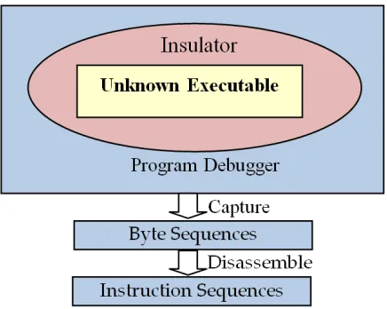
Figure 1 show dynamic instruction sequence capturing system we have built. The protection is provided by an insulator to ensure malicious behavior is contained. The
Figure 1. Dynamic Instruction Sequence Capturing System
protection is provided by hooking potentially destructive Win32 API functions. Instead of simply ignoring the func-tion and return failure to the caller, for most funcfunc-tions, we return success and invoke the function in a restrictive way to elicit more malicious behavior. For example, when a program requests a file handler with read/write permission, we return success and give the handler with read permission only. In this way, we can elicit malicious behavior as much as possible. Some viruses would stop execution if it detects failure of a particular system call.
The Win32 API functions protected by the protection mechanism include:
1) File/directory/registry manipulation API 2) Remote process/thread/memory manipulation 3) LoadLibrary/GetProcAddress
4) System administration API (system clock, etc) 5) Socket creation, packet sending
For category 3, we modify LoadLibrary / GetProcAd-dress because these API will load new dynamic mod-ules into the system. Our mechanism is based on the executable module and cannot control the behavior of these dynamic linked libraries. We use Microsoft detour library [9] to implement our protection mechanism.
However, some malicious program will invoke the un-derlying operating system native API in ntdll.dll or invoke interrupt 2e (or SysEnter/SysCall, on newer versions of Windows) directly, which is not protected by our system. A general solution for this problem is outside the scope of this paper.
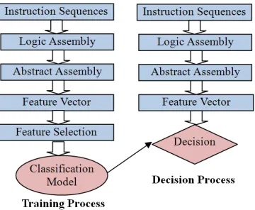
Figure 2. System Overview
III. SYSTEM OVERVIEW
Figure 2 shows the overview of our system. It in-cludes both the training process and the decision process. We have already discussed dynamic instruction collec-tion process before. So start from dynamic instruccollec-tion sequences, the training process derives logic assembly and abstract assembly. From abstract assembly, we can derive our feature vector. Through our feature selection and modeling process, we can build our classification model. On the end user side, we install a monitor system which will run unknown program under our protection mechanism as well. Based on the captured dynamic instruction sequences we run a decision process which derives logic assembly and abstract assembly, collects all the required features of the classification model, and uses these features to make our decision by the classification model.
Every classification model includes model parameters, feature set, and classifier. On the end user’s computer, models are constantly updated through an automatic up-date process. Latest models are built using the up to up-date virus and benign dataset to maintain the quality of the classification model. End user also has ability to change preferred model through a GUI, see Figure 3. In this dialog, 10 best models are sorted on accuracy (over testing dataset). The user can see how many instructions the model collects (n), what type of instruction association does it use (IAType), what is the classifier (model), how many features does it use (feature), what is false positive rate (fpr) and false negative rate (fnr).
IV. LOGIC ASSEMBLY
Our dynamic instruction capturing system captures execution log at a rate around 6,000 instructions per second in our computer. For some executable requiring interaction, we use the most straightforward way, such as typing ”enter” key in a command line application or press ”Ok” button in a GUI application to respond.
In a conventional disassembler, assembly instructions are organized into basic blocks. A basic block is a sequence of instructions without any jump targets in the middle. Usually disassembler will generate a label for
Figure 3. Model Selector
each basic block automatically. However, execution log generated by our system is simply a chronological record of all instructions executed. The instructions do not group into basic blocks and there are no labels. We believe that basic block capture the structure of instruction sequences and thus we process the instruction traces and organize them into basic blocks. We call the resulting assembly code ”logic assembly”.
Compared with static disassembler, dynamic captured instruction sequences may have incomplete code cover-age. This fact implies the following consequences about logic assembly code:
1) Some basic blocks may be completely missing 2) Some basic blocks may contain less instructions 3) Some jump targets may be missing, which makes
two basic blocks merge together
Despite these differences, logic assembly carries as much structural information of a program as possible.
We design the algorithm to construct logic assembly from runtime instructions trace. The algorithm consists of three steps and we describe below:
1) Sort all instructions in the execution log on their virtual addresses. Repeated code fragments will be ignored
2) Scan all jump instructions. If it is a control flow transfer instruction (conditional or unconditional), we mark it as the beginning of a new basic block 3) Output sorted instructions and labels if applicable We further prove that instructions inside a basic block are consecutive. Here consecutive means there is no hole inside address space representing the binary code of the basic block. If not, suppose there is a gap between adjacent instruction i1and i2inside the same basic block, then there must be a control flow transfer instruction j leads to i2, and j must be right before i2. So j should be in our chronicle instruction log as well. We will generate a new label for instruction i2. Then i1and i2are in different basic blocks, this contradicts our initial supposition.
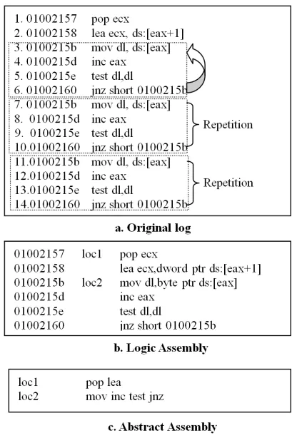
Figure 4. Logic Assembly and Abstract Assembly
the operands and prefix since the opcode represents the behavior of the program. The resulting assembly code is called abstract assembly [10].
Figure 4 shows an example of logic assembly and abstract assembly. Figure 4.a is the original instruction sequences captured by our system. We remove duplicated code from line 7 to line 14, and generate label for jump destination line 3. Figure 4.b is the logic assembly we generated. We further omit the operands and keep opcode, and we finally get abstract assembly Figure 4.c.
One merit of dynamic instruction sequences over con-ventional assembly is that dynamic instruction sequences expose some type of self-modifying behavior. If a pro-gram modifies its code at runtime, we may observer two different instructions at the same virtual address in runtime trace. A program may even modify its own code more than once. We devise a mechanism to capture this behavior while constructing logic assembly.
We associate an incarnation number with each vir-tual address we have seen in the dynamic instruction sequences. Initial incarnation number is 1. Each time we see an instruction at the same virtual address, we compare this assembly instruction with the one we have seen before at that virtual address, if the instruction changes, we incre-ment the incarnation number. Subsequent jump instruction will mark the beginning of a basic block on the newest incarnation. We treat instructions of different incarnations as different code segments, and generate basic blocks separately. Figure 5 illustrate this process. In this way we keep the behavior of any historical invocations even
Figure 5. Different Incarnations
the code is later overwrote by newly generated code.
V. INSTRUCTION ASSOCIATIONS
we get abstract assembly, we are interested in finding relationship among instructions within each basic block. We believe the way instruction sequences groups together within each block carries the information of the behavior of an executable.
The instruction sequences we are interested in are not limited to consecutive and ordered sequences. Virus writers frequently change the order of instructions and insert irrelevant instructions manually to create a new virus variation. Further, metamorphism viruses [3] au-tomatically change the order of sequences and insert garbage among useful instructions to make new virus copies. The resulting virus variation still exhibits the malicious behavior. However, any detection mechanism based on consecutive and ordered sequences such as N-Gram could be fooled.
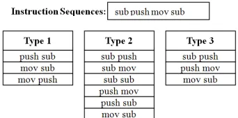
We have two considerations to obtain the relationship among instructions. First, whether the order of instruc-tions matters or not; Second, whether the instrucinstruc-tions should be consecutive or not. Based on these two criteria, we use three methods to collect features.
1) The order of the sequences is not considered and there could be instructions in between
2) The order of instructions is considered, it becomes instruction episodes. However, it is not necessary for instruction episodes to be consecutive
3) The instructions are both ordered and consecutive We call these ”Type 1”, ”Type 2” and ”Type 3” instruction associations. ”Type 3” instruction association is similar to N-Gram. ”Type 2” instruction association can deal with garbage insertion. ”Type 1” instruction association can deal with both garbage insertion and code reorder.
Figure 6 illustrates different type of instruction asso-ciations of length 2 we have obtained on an instruction sequence consisting of 4 instructions.
VI. DATA MINING PROCESS
Figure 6. Example for instruction associations of length 2
Figure 7. Data Mining Process
1) Run executable inside a virtual machine, obtain instruction sequences from our system
2) Construct logic assembly 3) Generate abstract assembly 4) Feature selection
5) Generating training dataset and testing dataset 6) Build classification models
7) Evaluation
This process is illustrated in Figure 7.
Here we describe step 4 in detail. The features for our classifier are instruction associations. To select ap-propriate instruction associations, we use the following two criteria:
1) The instruction associations should be frequent in the training dataset consisting of both benign and malicious executables. If it occurs very rarely, we would rather consider this instruction association is a noise and not use it as our feature
2) The instruction associations should be an indicator of benign or malicious code; In other words, it should be abundant in benign code and rare in malicious code, or vice versa
To satisfy the first criteria, we only extract frequent in-struction associations from training dataset. Only frequent instruction associations can be considered as our feature. We use a variation of Apriori algorithm [11] to generate all three types of frequent instruction associations from abstract assembly. Although there exist algorithms to optimize Apriori algorithm [12], the optimization only applicable to type 1 instruction association, besides, this step only occurs at training time. We believe optimize decision process is more critical because it will run on each end user computer under protection. Training, however, only need to be done on some specific server
computers.
One parameter of Apriori algorithm is ”minimum sup-port”. It is the minimal frequency of frequent associations among all data. More specifically, it is the minimum percentage of basic blocks that contains the instruction sequences in our case. We do experiments on different support level as described in section VIII.
To satisfy the second criteria, we define the term contrast:
Contrast(F i) =
countB(F i)+ε
countM(F i)+ε countB(F i)≥countM(F i) countM(F i)+ε
countB(F i)+ε countB(F i)< countM(F i) .
BCount (Fi) normalized count of Fi in benign instruction file
MCount (Fi) normalized count of Fi in malicious instruction file
ε a small constant to avoid error when the
denominator is 0
In this formula, normalized count is the frequency of that instruction sequence divided by the total number of basic blocks in abstract assembly. We use a slightly larger benign code dataset than malicious code dataset. The use of normalization will factor out the effect of unequal dataset size.
We select top L features as our feature set. For one executable in training dataset, we count the number of basic blocks containing the feature, normalized by the number of basic blocks of that executable. We process every executable in our training dataset, and eventually we generate the input for our classifier.
We use two classifiers in our experiments: decision tree and Support Vector Machine.
Decision tree is a classification algorithm that is con-structed by recursively splitting the dataset into parts. Each such split is determined by the result of the entropy gain of all possible splits among all attributes inside the tree node. The decision tree keeps growing as more splits are performed until a specific stop rule is satisfied. During postpruning, some splits are removed to reduce overfitting problem. When a record of an unknown class comes in, it is classified through a sequence of nodes from the tree root down to the leaf node. Then, it is labeled by the class the leaf node represents. We use Quinlan’s c4.5 decision tree [13] as our decision tree implementation.
Support Vector Machine (SVM) [14] is essentially a mathematical optimization problem which is originated from the linear discriminant problem. However, if two classes are inseparable in two dimensions, SVM can use a mapping, which is called kernel function, to map two dimension data into a higher dimension. The two classes may be separable in higher dimension. libSVM [15] is a popular C implementation of SVM on Unix.
VII. PERFORMANCE ANALYSIS
In this section, we focus on average performance when applying the classification model on the end user computer. The performance to process one unknown executable is determined by the following factors:
1) Capturing instruction sequences 2) Generating logic assembly
3) Counting the occurrence of instruction associations in feature set to generate feature vector
4) Applying classification model
Unlike system calls, instruction sequences are gener-ated fast and at a relative stable rate. On our test computer, we generate average 6,000 instruction sequences in 1 second under our system. That is enough for the input for our classifier. This is one advantage over system call approach, which takes more time to collect enough traces. However, instruction sequences collection rate is not really stable. We could spend much more than aver-age time to capture instruction sequences. For example, some system calls will block the process so we cannot capture any instructions for this program module during system call. Some program will wait for user’s response to continue executing. To solve this problem, we also specify a time limit on instruction capturing. We will stop capturing instruction sequences and continue to the next step whenever a timeout occurs.
Generating logic assembly consists of three phases. In the first phase, we need to sort the instruction sequences according to their virtual address. This could take up to O(nlogn) to finish. In the second phase, we mark jump destination using one linear scan of all instructions, which takes O(n). Maintaining different incarnations requires a memory map to remember the instruction and incarnation of each virtual address. Every instruction takes linear time to check this memory map, so this additional task will not increase the order of the overall processing time. Finally, we traverse the sorted instruction list to output basic blocks, which takes O(n). So the overall time complexity in logic assembly generation is O(nlogn).
Generating features vector requires counting the fre-quency of L features. Suppose one basic block contains average k instructions, thus we have average n/k basic blocks. For every basic block, we will do a search for each one of L features.
Different types of instruction association require differ-ent approaches to search inside a basic block. For type 1 instruction association, we use an occurrence bit for every instruction in the association, if all bit is on, then the basic block contains that instruction association. For type 2, we construct a finite state machine (FSM), and scan the basic block from the beginning. If we encounter an instruction matching the state in FSM, we change the state of FSM, and begin matching the next instruction. For type 3, it is similar to a substring search. All these three types of search requires one linear scan of the basic block, makes the average complexity O(k).
We can calculate the processing time of feature vector generation as the product of the above factors. So this step
takes (search time per feature per basic block)* (feature number) * (basic block number) = O(n/k*k*L) = O(nL). The time complexity to apply a classifier is a property of that specific classifier.
For C4.5 decision tree, the applying time complexity is proportional to the depth of the tree [13], which is a constant at the decision time. SVM takes O(L) time to apply the model on a specific feature vector [17].
Based on the discussion above, we conclude that the av-erage time complexity to process an unknown executable is bounded by max (O(nlogn), O(nL)), in which n is the number of instructions captured, L is the number of features.
In our experiment, processing instructions captured in 1 second, for which n≤6000, the calculation time is usually less than 3 seconds. This suggests that this approach can be used in practice.
VIII. EXPERIMENTAL RESULTS
A. Dataset
Due to the prevailing dominance of Win32 viruses today, we use Win32 viruses as our virus dataset. We collect 267 Win32 viruses from VX heaven [18].
We also choose 368 benign executables which consist of Windows system executables, commercial executables and open source executables. These executables have similar average size and variation as the malicious dataset. Some viruses fail to execute fully and we can only collect less than 10 dynamic instructions. We exclude these viruses from our dataset due to lack of enough information for further processing. By manually analyzing these viruses, we found that these viruses quit early due to failure to identify or execute some system functions. This is usually due to the virus author making false assumption about the operating system which is not present in the destination system. For example, Win32.Alcaul.b is trying to write to a read only page at 5th instruction. While it is possible in earlier version of Windows, current version of Windows correct the problem and this operation is no longer possible. The virus code quit quickly due to access violation. All such viruses we have encountered are not actually presenting malicious behavior before they quit and thus would not destroy end user computer. So we believe ignoring these viruses in our system would not cause a big problem.
B. Criteria
is the proportion of benign executables that were erro-neously reported as being malicious. On contrary, false negative rate is the proportion of malicious executables that were erroneously identified as benign. We believe in a virus detection mechanism, low false negative rate is more vital than low false positive rate. It is wise to be more cautious against those suspicious unknown executables. High false positive certainly make things inconvenient for the user, but high false negative will destroy a user’s computer, which is more harmful.
C. Parameter Selection
There are five primary parameters in our classifier, they are:
1) Instruction association type IA (type 1, 2 or 3) 2) Support level of frequent instruction association (S),
we experiment with 0.003, 0.005, 0.01
3) Number of features (L), we try 10, 20, 50, 100, 200, 300. At some support level, some instruction association type generates relatively fewer number of available features. For example, at support lever 0.01, only 23 type 1 instruction associations are frequent. In that case, we use up to the maximum available features
4) Type of classifier (C), we compare C4.5 decision tree and SVM (Support Vector Machine)
5) Number of instruction captured (N). We try 1000, 2000, 4000, 6000, 8000
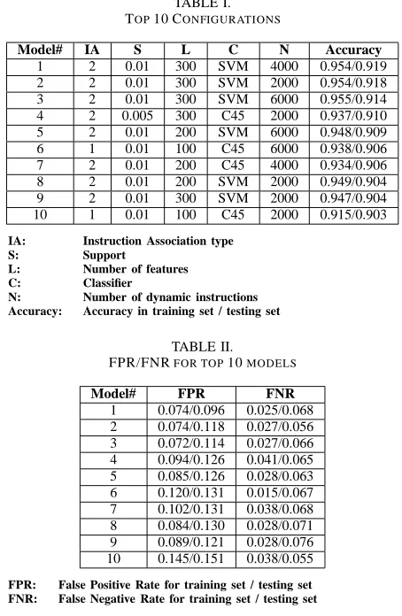
Table I list top 10 configurations we get along with training and testing accuracy. Table II is their according false positive rate and false negative rate.
The result shows that support level 0.01 is clearly superior to others. That shows that frequent patterns are more important than infrequent patterns.
Instruction association type 1 and 2 outperform type 3. That is an interesting result which could serve to justify our approach over traditional N-Gram based approach in that N-Gram checks consecutive and ordered sequence only.
The performance of SVM is a little bit better than C4.5 in our top 10 list. The average testing accuracy of SVM in top 10 models is 0.911 compared with 0.906 of C4.5. Figure 8 shows the effect of number of feature L vs average accuracy among all models. Generally, more features give more accurate result. However, the margin is small after L>100. Larger feature number implies longer processing time for monitor system. Usually 200-300 features are optimal.
The effect of number of instructions captured N is not quite clear yet. We further calculate average accuracy at different N in Figure 9. We see that generally accuracy increases when we use a large N. However, the difference becomes very small when N>2000, especially for testing dataset. That justifies that when we use the initial part of instructions, we can capture the behavior of the unknown executable. One interesting phenomenon is when N=2000, we get some really good result. Half of our top 10 models use 2000 instruction sequences. That means in
Figure 8. Effect of L
Figure 9. Effect of N
some settings, first 2000 instructions already capture the character of the executable, further instructions might only give noise.
D. Decision Process
Table III shows typical processing time to process one unknown program in seconds on our test computer. The test computer has a typical configuration of recent personal computer with 1 AMD Turion 1.58G CPU and 1G memory. ”Log” is the time to capture necessary instruction sequences. ”Assembly” is the time to construct logic assembly and then get abstract assembly. ”Feature” is the time to extract feature vector. ”Model” is the time needed to apply the classifier. Table IV is normalized execution time divided into different components.
TABLE I. TOP10 CONFIGURATIONS
Model# IA S L C N Accuracy
1 2 0.01 300 SVM 4000 0.954/0.919
2 2 0.01 300 SVM 2000 0.954/0.918
3 2 0.01 300 SVM 6000 0.955/0.914
4 2 0.005 300 C45 2000 0.937/0.910
5 2 0.01 200 SVM 6000 0.948/0.909
6 1 0.01 100 C45 6000 0.938/0.906
7 2 0.01 200 C45 4000 0.934/0.906
8 2 0.01 200 SVM 2000 0.949/0.904
9 2 0.01 300 SVM 2000 0.947/0.904
10 1 0.01 100 C45 2000 0.915/0.903
IA: Instruction Association type
S: Support
L: Number of features C: Classifier
N: Number of dynamic instructions Accuracy: Accuracy in training set / testing set
TABLE II.
FPR/FNRFOR TOP10MODELS
Model# FPR FNR 1 0.074/0.096 0.025/0.068 2 0.074/0.118 0.027/0.056 3 0.072/0.114 0.027/0.066 4 0.094/0.126 0.041/0.065 5 0.085/0.126 0.028/0.063 6 0.120/0.131 0.015/0.067 7 0.102/0.131 0.038/0.068 8 0.084/0.130 0.028/0.071 9 0.089/0.121 0.028/0.076 10 0.145/0.151 0.038/0.055
FPR: False Positive Rate for training set / testing set FNR: False Negative Rate for training set / testing set
Other time components are relatively stable. SVM model takes significantly more time than C4.5.
The overall processing time is usually under 3 seconds. We also tested the capacity of our malicious behavior protection system. We run all 267 malicious programs from our dataset inside our monitor system. None of them present obvious malicious behavior. Although our protec-tion scheme is not complete as discussed in secprotec-tion II, most viruses are well guarded by our system.
IX. RELATED RESEARCH
Although the problem of determining whether an un-known software is malicious or not has been proven to be generally undecidable [19], detecting viruses with an acceptable detecting rate is still possible. A number of approaches have been proposed to detect unknown viruses.
Static approach checks executable binaries or assembly code without actually executing the unknown program.
The work of Arnold et al [20] uses binary trigram as their detecting criteria. They use neural network as their classifier and reported a good result in detecting boot sector viruses for a small sample size.
InSeon et al [21] also use binary sequences as features. However, they construct a self organizing map on top of these features. Self organizing map converts binary sequences into a two dimensional map. They claim that
TABLE III.
TYPICALRUNTIME FORMONITORSYSTEM
Model# Total Log Assembly Feature Model
1 1.79 0.25 0.06 0.37 1.12
2 1.66 0.22 0.03 0.13 1.28
3 2.86 0.34 0.08 1.24 1.20
4 0.34 0.15 0.03 0.14 0.02
5 2.29 0.36 0.09 0.85 1.02
6 0.45 0.35 0.08 0.02 0.01
7 0.56 0.27 0.05 0.23 0.01
8 1.29 0.18 0.03 0.10 0.99
9 1.44 0.27 0.03 0.13 1.01
10 0.23 0.19 0.07 0.01 0.01
TABLE IV.
NORMALIZEDRUNTIME FORMONITORSYSTEM
Model# NLog NAssembly NFeature NModel
1 0.06 0.015 0.031 0.37
2 0.11 0.015 0.021 0.42
3 0.06 0.013 0.069 0.40
4 0.08 0.015 0.023 /
5 0.06 0.015 0.071 0.51
6 0.06 0.013 0.003 /
7 0.07 0.013 0.029 /
8 0.09 0.015 0.025 0.50
9 0.14 0.015 0.022 0.50
NLog = Log Time / 1000 Instructions NAssembly = Assembly Time / 1000 Instructions
NFeature = Feature Selection Time / (100 Features * 1000 Instructions) NModel = SVM Classification Time / 100 Features
malicious viruses from the same virus family demonstrate the same characteristic in the resulting graph. But they do not give a quantitative way to differentiate a virus from benign code.
Schultz et al [22] use comprehensive features in their classifiers. They use three groups of features. The first group is the list of DLLs and DLL function calls used by the binary. The second group is string information acquired from GNU strings utility. The third group is a simple binary sequence feature. They conducted exper-imentation using numerous classifiers such as RIPPER, Naive Bayes and Multi-Naive Bayes.
In recent years, researchers start to explore the possi-bility to use N-Gram in detecting computer viruses [23]– [25]. Here N-Gram refers to consecutive binary sequences of fixed size inside binary code.
Kolter et al [25] extracted all N-Gram from a training set and then performed a feature selection process based on information gain. Top 500 N-Gram features are se-lected. Then, they mark the presence of each N-Gram in the training dataset. These binary tabular data are used as the input data for numerous classifiers. They exper-imented with Instance-based Learner, TFIDF classifier, Naive Bayes, Support Vector Machines, Decision Trees and Boosted Classifiers. Instead of accuracy, they only reported AUC (Areas Under Curves). The best result is achieved by boosted J48 at AUC, 0.996.
information to understand its behavior. We redid the experiment mentioned in [25] and we found that the key contributors that lead to the classifications are not from bytes which representing virus code, rather, they are from structural binary or string constants. Since structural binary and string constants are not essential components to a virus, this suggests that those detection mechanisms can be evaded.
Another area of current researches focuses on higher level features constructed on top of assembly code.
Sung A.H.et al [26] proposes to collect API call sequences from assembly code and compare these se-quences to known malicious API call sese-quences.
Mihai et al [27] uses template matching against as-sembly code to detect known malicious behavior such as self-modification.
In [28], the author proposed using control graph ex-tracted from assembly code and then use graph comparing algorithm to match it against known virus control graphs. These approaches seem to be promising. The problem is that disassembling executable code itself is a hard problem [29]–[31].
Besides static analysis, runtime features have also been used in virus research. Most of current approaches are based on system calls collected from runtime trace.
TTAnalyze [32] is a tool to execute an unknown executable inside a virtual machine, which captures all system calls and parameters of each system call to a log file. An expert can check the log file to find any malicious behavior manually.
Steven A. Hofmeyr et al [33] proposes one of the very first data mining approaches using dynamic system call. They build an N-Gram system call sequences database for benign programs. For every unknown executable, they obtain system call sequences N-Grams and compare it with the database, if they cannot find a similar N-Gram, then the detection system triggers alert.
In [34], the author proposes several data mining ap-proaches based on system calls N-Gram as well. They try to build a benign and malicious system call N-Gram database, and obtain rules from this database. For unknown system call trace, they calculate a score based on the count of benign N-Gram and malicious N-Gram. In the same paper, they also propose an approach to use first (n-1) system calls inside N-Gram as features to predict the nth system call. The average violation score determines the nature of the unknown executable.
In [35], the author compares three approaches based on simple N-Gram frequency, data mining and hidden Markov model (HMM) approach, and conclude that though HMM is slow, it usually leads to the most accuracy model.
In [36], the author runs viruses executables inside a vir-tual machine, collecting operating system call sequences of that program. The author intends to cluster viruses into groups. The author uses k-medoid clustering algorithm to group the viruses, and uses Levenshtein distance to calcu-late the distance between operating system call sequences
of different runtime traces.
[37] is the most similar research with ours. The major difference between [37] and this paper is that we are using runtime features rather than static features of a program.
X. CONCLUSION
In this paper, we have proposed a novel malicious code detection approach by mining dynamic instruction sequences and described experiments conducted against recent Win32 viruses within a monitored system. This monitor system designed in this work can be installed easily by an ordinary user.
Experimental results indicate that the proposed data mining approaches can detect malicious codes reliably for the unknown computer viruses. The accuracy of the top the classification models ranges from 90% to 92%.
Compared with other approaches, instruction associa-tion deals with the virus code directly and is hard to evade by virus writer.
Since we are conducting our experiments by executing a finite number of instructions from the begining, our method will not detect any malicious code hooked in the remaining part of the executable code. In addition, since we follow one possible executable path, it is possible to miss malicious section of code in our experiment.
Our experiments show that dynamic approaches alone cannot solve the detection problem with guarantee. We expect by combining both static and dynamic approaches might provide a better detection result. We plan to explore this area in our future work.
REFERENCES
[1] Microsoft Antimalware Team, “Microsoft Security Intelli-gence Report (January - June 2007),” 2007.
[2] C. Nachenberg, “Computer virus-antivirus coevolution,”
Communications of the ACM, vol. 40, no. 1.
[3] P. Szor and P. Ferrie, “Hunting for metamorphic,” in 11th
International Virus Bulletin Conference, 2001.
[4] Jeffrey O. Kephart, William C. Arnold, “Automatic Ex-traction of Computer Virus Signatures,” in Virus Bulletin
International Conference, 1994.
[5] http://zert.isotf.org/.
[6] Peter Szor, THE ART OF COMPUTER VIRUS
RE-SEARCH AND DEFENSE. Addison Wesley, 2005. [7] Jiawei Han, Micheline Kamber, Data Mining: Concepts
and Techniques. Morgan Kaufmann Publishers, Mar. 2006.
[8] http://www.vmware.com.
[9] http://research.microsoft.com/sn/detours/.
[10] Md. Enamul. Karim et al, “Malware Phylogeny Genera-tion using PermutaGenera-tions of Code,” Journal in Computer
Virology, vol. 1, no. 1-2, Nov. 2005.
[11] Rakesh Agrawal, Ramakrishnan Srikant, “Fast Algorithms for Mining Association Rules,” in Proc. 20th Int. Conf.
Very Large Data Bases(VLDB), 1994.
[12] Jiawei Han , Jian Pei , Yiwen Yin, “Mining frequent patterns without candidate generation,” in Proceedings
of the 2000 ACM SIGMOD international conference on Management of data, 2000.
[13] J.R.Quinlan, C4.5:Programs for Machine Learning. Mor-gan Kaufmann, 1993.
[14] John Shawe-Taylor and Nello Cristianini, Support Vector
[15] http://www.csie.ntu.edu.tw/ cjlin/libsvm.
[16] Breiman, L., “Random Forests,” Machine Learning, vol. 45, pp. 5–32.
[17] Vladimir Vapnik, Statistical Learning Theory. Wiley, 1998.
[18] http://vx.netlux.org.
[19] F. Cohen, “Computational Aspects of Computer Viruses,”
Computers and Security, vol. 8, pp. 325–344, 1997.
[20] William Arnold, Gerald Tesauro, “Automatically generated Win32 heuristic virus detection,” in Virus Bulletin
confer-ence, Sept. 2000.
[21] InSeon Yoo, “Visualizing windows executable viruses us-ing self-organizus-ing maps,” in Proceedus-ings of the 2004 ACM
workshop on Visualization and data mining for computer security, Oct. 2004.
[22] Matthew G. Schultz, Eleazar Eskin, Erez Zadok, and Salvatore J. Stolfo, “Data Mining Methods for Detection of New Malicious Executables,” in Proceedings of IEEE
Symposium on Security and Privacy, May 2001.
[23] Tony Abou-Assaleh, Nick Cercone, Vlado Keselj, and Ray Sweidan, “Detection of New Malicious Code Using N-grams Signatures,” in Proceedings of the Second Annual
Conference on Privacy, Security and Trust (PST’04), Oct.
2004, pp. 193–196.
[24] Abou-Assaleh, Nick Cercone, Vlado Keselj, and Ray Sweidan, “N-Gram-based Detection of New Malicious Code,” in Proceeding of the 28th Annual International
Computer Software and Applications Conference (COMP-SAC’04), 2004.
[25] Kolter, J.Z., and Maloof, M.A, “Learning to detect mali-cious executables in the wild,” in Proceedings of the Tenth
ACM SIGKDD International Conference on Knowledge Discovery and Data Mining, 2004, pp. 470–478.
[26] Sung, A.H et al, “Static analyzer of vicious executables (SAVE),” in 20th Annual Computer Security Applications
Conference, 2004.
[27] Mihai Christodorescu, Somesh Jha, Sanjit A. Seshia, Dawn Song, Randal E. Bryant, “Semantics-Aware Malware De-tection,” in IEEE Symposium on Security and Privacy, 2005.
[28] Mihai Christodorescu, Somesh Jha, “Static Analysis of Executables to Detect Malicious Patterns,” in 12th USENIX
Security Symposium, 2003.
[29] Christopher Kruegel et al, “Static Disassembly of Obfus-cated Binaries,” in Proceedings of the 13th conference on
USENIX Security Symposium, 2004.
[30] Cullen Linn et al, “Obfuscation of Executable Code to Improve Resistance to Static Disassembly,” in Proceedings
of the 10th ACM conference on Computer and communi-cations security, Oct. 2003.
[31] B. Schwarz, S. Debray, G. Andrews, “Disassembly of Executable Code Revisited,” in Ninth Working Conference
on Reverse Engineering (WCRE 2002), 2003, p. 0045.
[32] Bayer, U., Kruegel, C., Kirda, E, “TTAnalyze: A Tool for Analyzing Malware,” in EICAR. 15th Annual Conference
of the European Institute for Computer Antivirus Research,
2006.
[33] Steven A. Hofmeyr et al, “Intrusion detection using se-quences of system calls,” Journal of Computer Security, vol. 6, no. 3, 1998.
[34] Wenke Lee and Salvatore J. Stolfo, “Data Mining Ap-proaches for Intrusion Detection,” in 7th USENIX Security
Symposium, 1998.
[35] Warrender, C et al, “Detecting intrusions using system calls: alternative data models,” in Proceedings of the 1999
IEEE Symposium on Security and Privacy, 1999.
[36] Tony Lee, Jigar J. Mody, “Behavior Classification,” Mi-crosoft Antivirus team, 2006.
[37] Muazzam Ahmed Siddiqui, “DATA MINING METHODS
FOR MALWARE DETECTION,” University of Central Florida, Tech. Rep., 2008, phD Dissertation.
Jianyong Dai received a MS in Computer Science from Univer-sity of Central Florida in 2008, and a BS in Computer Science from Shanghai Jiaotong University, Shanghai, China in 1998. He is pursuing his doctorate study in Computer Science in the School of Computer Science at the University of Central Florida. His research interests include security, data mining and parallel and distributed computing.
Ratan Guha is a Professor of Computer Science at the University of Central Florida, Orlando. His research interests include distributed systems, computer networks, security pro-tocols, modeling and simulation, and computer graphics. His research has been supported by grants from the US Army Research Office, US National Science Foundation, STRICOM, PM-TRADE, and the State of Florida. He is a life member of IEEE, IEEE Computer Society, IEEE Communication Society, and a member of ACM.