A novel revenue optimization model to address the operation and maintenance cost of a data center

R E S E A R C H

Open Access

A novel revenue optimization model to

address the operation and maintenance cost

of a data center

Snehanshu Saha

, Jyotirmoy Sarkar

, Avantika Dwivedi

, Nandita Dwivedi

, Anand M. Narasimhamurthy

and Ranjan Roy

Abstract

Enterprises are enhancing investments in cloud services setting up data centers to meet growing demand. A typical investment is of the order of millions of dollars, infrastructure and recurring cost included. This paper proposes an algorithmic/analytical approach to address the issues of optimal utilization of the resources towards a feasible and profitable model. The economic sustainability of such a model is accomplished via Cobb-Douglas production function. The production model seeks to answer questions on maximal revenue given a set of budgetary constraints. The model suggests minimum investments needed to achieve target output.

Keywords: Cobb-Douglas production function, Data center, Concavity, Returns to scale, Profit function, Cost function

Motivation and background

IT operations are integral to most business organizations around the world. The business communities need to rely on the information systems to run their organiza-tional operations. Therefore, a company may incur loss due to disruptions and unavailability of information sys-tems. It is necessary to have an IT infrastructure, which houses all the information systems to minimize all kind of disruptions and obstacles related to information sys-tems. This reliable IT infrastructure is called data center. The cost to run a data center is generally associated with power, cooling, networking and storage equipment. A data center houses thousand of information and com-puting systems deployed in computer racks. A rack is an Electronic Industries Association enclosure, which is 2 meters high, 0.61 meters wide and 0.76 meters deep. A standard rack accommodates 40-42 computing units and dense rack configuration servers (Blade rack) will accom-modate 200 computing units. The heat dissipated by a standard rack is 10 KW and Blade rack will dissipate heat up to 30 KW. Hence, a data center containing 2000 racks

*Correspondence: [email protected]

1Center for Applied Mathematical Modeling and Simulation (CAMMS) & Department of Computer Science and Engineering, PESIT-BSC, Bangalore, 560100, India

Full list of author information is available at the end of the article

may require 20 MW power [1]. Increasingly, PC-based computing and storage services are relocating to Inter-net services. While early InterInter-net services were mostly informational, many recent Web applications offer ser-vices that previously resided in the client, including email, photo and video storage and office applications. The shift from PC-based computing services to server-side comput-ing is driven primarily not only for the improvements in services, such as the ease of management (no configura-tion or backups needed) and ubiquity of access (a browser is all you need), but also by the advantages it offers to ven-dors. Now a days, Software as a service provides faster application development because it is easier for software vendors to make changes and improvements. Instead of updating millions of clients, vendors need to coordinate improvements and fixes inside their data centers and can restrict hardware deployment to a few well-tested config-urations. Moreover, data center economics allows many application services to run at a low cost per user. For example, servers may be shared with thousands of active users (and many more inactive ones), resulting in better utilization. Similarly, the computation itself may become cheaper in a shared service (e.g., an email attachment received by multiple users can be stored once rather than many times). Finally, servers and storage in a data cen-ter can be easier to manage than the desktop or laptop

equivalent because they are under the control of a single, knowledgeable entity [2]. Though each data center is dif-ferent based on the operations, facilities and the average cost per year to operate, a large data center costs between $10 million to $25 million. 42 % of costs are associated with hardware, software, uninterrupted power supplies, and networking. 58 % of the expenses is due to heating, air conditioning, property and sales tax. In a traditional data center, most of the cost is consumed by infrastructure for maintenance. A few surveys have estimated the mainte-nance cost up to 80 % of the total cost. As data centers have become important aspects in business organization, it is imperative to examine the cost-revenue dynamics and design an effective way to optimize it. Cisco in its Global Cloud Index (GCI) Reports-2012, forecasted data center traffic to shoot up to 554 exabytes (EB) per month by 2016, from 146 exabytes. There are a few techniques to optimize cost and profit. Cobb-Douglas is a widely used production model, but to the best of our knowledge, has never been used in the study of optimization issues arising in data centers.

Introduction & overview

The authors find it necessary to discuss different aspects of data centers and optimization, before proceeding to relevant scholarly work available in the public domain.

Data center key subsystems

A data center consists of many subsystems. Three main subsystems would be discussed here. These are often referred as ‘Power, Ping, and Pong’, required to run a data center [1].

1. Continuous power supply. 2. Air conditioning.

3. Network Connectivity.

Power is essential to provide uninterrupted services throughout the year. At large data centers, electricity is supplied either from a grid or from on-site generators. The electricity supplied to the computer racks is dissipated as heat. Therefore, a cooling system is required to mitigate the heat. Generally data centers have chillers to supply cold water, which is used for air conditioning. Network connectivity is necessary for data transmission within and outside of a data center. The power subsystem consists of a grid and backup generator. The network subsystems com-prise of all the connectivity except rack switches, whereas cooling subsystem includes chiller and air conditioning system.

Traditional data center

Running a traditional data center is expensive in com-parison to a cloud data center. Thousands of applica-tions are running in traditional data centers along mixed

hardware tool. Maintaining existing infrastructure con-sume the biggest chunk of the total cost and multiple management tools are required for operation and man-agement. Lately, traditional data centers are being used by internet service providers for housing their own or third party servers. Traditionally data centers were either con-structed for meeting the purpose of large organizations or Network-neutral data centers. These facilities establish interconnection of carriers and act as regional fiber hubs, providing services to local business in addition to hosting content servers.

Cloud data center

Cloud data center is a place, where 10,000 or more servers are hosted to provide services for applications. Consistent infrastructure components like racks, hardware, OS, net-working etc. are generally used to build the cloud data center. One of the important features of cloud data cen-ter is that they are not remodeled traditional data cencen-ters. Salient features of cloud data centers are listed below:

• Constructed for serving different objectives.

• Built to a different scale.

• Created at a different time than the traditional data center.

• Unlike traditional data center, these are responsible for executing and managing different workload.

• Not constrained by limitations of traditional data centers.

The cost associated with cloud data centers are com-posed of three factors. Labor cost takes the smallest chunk of total operation cost, nearly 6 % of the total cost, whereas power and cooling cost and computing costs are 20 % and 48 % respectively. Other costs account for remaining 26 %. Cloud data centers add new cost, unlike traditional data centers [3].

Data center tiers

Data centers have been divided based on the destination available; each data center has been modeled for address-ing specific business requirement and has operational problems and issues for various reasons:

• Data centers related to Corporate house.

• Data centers responsible for computer infrastructure as a service (IaaS) and hosting Web application.

• Data centers that provide services of TurnKey Solutions

• Data centers, where Web 2.0 has been implemented.

Data center optimization

leadership thinks of the data center as a factory-like utility that collects and processes information. Top management understands the value of data that’s available in real time to help inform and shape decision-making. They also expect the data center to be fast enough to adopt new, rapidly deployed, public facing and internal user appli-cations. From a technology standpoint, data center of today must support mobility, provisioning on demand, scalability, virtualization and the flexibility to respond to fast-changing operational situations. From an economic standpoint, a few years of edgy fiscal conditions have imposed tight budgets on IT organizations in both the public and private sectors. That’s the reason behind new thinking being introduced in data center modeling and management. Organizations expect maximum output for every dollar invested in IT. They also face pressure to reduce power usage as a component of overall organiza-tional strategies for reducing their carbon footprint [4]. The challenges any data center faces in power consump-tion are listed below

• Lack of Access to Basic Data: Accurate data is required for achieving short-term and long-term capacity planning to ensure organizations don’t overinvest or underinvest in power and cooling infrastructure. Specifically, IT industries need the ability to keep track of individual and aggregated server power usage and temperature data at any point of time and historical trends as well.

• Inefficient Use of Power: Server power is typically over allocated and racks are under populated in worst-case. This may create a situation where power infrastructure is inefficiently used and contributes to overinvestment in racks and power capacity. IT solutions need to figure out a mechanism to control power consumption below theoretical peak values so

that kilowatt capacity of each rack may be fully utilized.

• Power and Cooling Excursions: The availability of services during business-critical time is a top priority though power supply disruption or cooling tower failures can affect business operations massively. IT must be able to survive such failures to avoid downtime and deliver reliably on service level agreements (SLAs).

• Higher density endowed computing environments are more efficient but can lead to localized hot spots during periods of peak utilization. Organizations need to identify and mitigate hot spots and optimize workload placement based on power and cooling availability and efficiency [5].

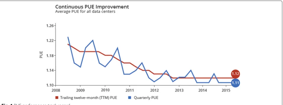
Rising energy costs and environmental responsibility have placed the data center industry under increasing pres-sure to improve its operational efficiency. According to Koomey, data center consumed 1.3 % of the global energy usage in 2010 [6]. At this scale, even relatively small effi-ciency improvements will result in significant cost savings and prevent millions of tons of carbon emissions. Google and other major Internet companies have made signif-icant contributions towards improving the data center efficiency. The overall pace of PUE reduction has slowed down,given diminishing returns and the limitations of ex-isting cooling technology [7]. Furthermore, best practice techniques such as hot air containment, water-de econo-mization and extensive monitoring are now commonplace in largescale data centers [8]. Figure 1 shows Google’s PUE performance track record from an annualized fleetwide PUE of 1.21 in 2008 to 1.12 in 2013, due to the imple-mentation of best practices and natural progression down the learning curve [9]. Note the asymptotic decline of the trailing twelvemonth (TTM) PUE graph [10].

In this paper, we propose a revenue model, which is best suited for the data centers in the current scenario. Mathe-matically, we have established the relevance of the model with the data centers. We find Cobb-Douglas model (CD) to be most suitable for optimizing the cost associated with the data centers. 3D graphs of cost data collected from various sources, have been generated for better under-standing of the model. The remainder of the paper is orga-nized as follows: Related work in the same field by other authors and Industry practices have been discussed in Section Introduction & overview. The analytical founda-tion of our proposed decision model has been elaborated in Section Related work. The decision model has been applied on data center’s real time data set and results have been analyzed in Section Analytical foundations of the decision model. We have compared our model with other mathematical models used in data center and explored the ways to overcome the drawbacks of CD function in conclusion Section Results and discussion. Appendix contains the mathematical proofs of optimal revenue and cost, computation of elasticities and relevant Matlab codes.

Related work

Industry practices

Enterprises make investments in millions of dollars on setting up data centers. The elite list includes many Fortune 500 companies Google, Apple, Facebook Inc., Amazon.com, and Microsoft, to name a few. Each of the four new Google data center projects unveiled in 2007, cost an estimated $600 million, which includes capital investment for construction, infrastructure, and servers for two data center buildings. In its earnings reports, Google reported $1.9 billion spent on data centers in 2006 and $2.4 billion in 2007 [11]. Apple operates a data center in Newark, California, which it acquired in 2006 for approximately $45 million at a significant discount to its construction cost. The data center occupies 108,000 square feet of total space. Apple intends to invest more than $1 billion over the next 10 years on its 183-acre data center campus in Maiden, North Carolina [12]. Facebook has invested more than $1 billion in the infrastructure that powers its social network, which now serves more than 845 million users a month around the globe. The com-pany spent $606 million on servers, storage, network gear and data centers in 2011, and spent another $500 million in 2012 [13]. In his research at Microsoft and Amazon Web Services, Hamilton has focused on cost models for operating hyper-scale data centers. His presentation at the Amazon open house reviewed cost assumptions for an 8 megawatt data center, which could include 46,000 servers. The cost was estimated at $88 million (about $11 million per megawatt), inclusive of monthly operating costs for a

facility, which is dominated by the cost for servers (57 %), followed by power and cooling (18 %) and electric power (13 %) [14].

A similarity between cloud and traditional data cen-ter is that both can be used for data storage. Cloud is an example of off-premises computing, whereas data centers are being used on premise storing system. Nowa-days, data centers are effectively being utilized in cloud computing. Cloud services are now being provided through data centers, which house cloud services and cloud-related resources. Cloud service providers also own data centers, which is located in different geographi-cal location, for provisioning of uninterrupted services in case of outage and unpredictable situations. IaaS (Infrastructure as a service), which provides facilities like virtual machines, storage and load balancing maintains a large pool of resources in data centers. Data centers, which are largely being used for cloud computing are called cloud data center. Lately the demarcation of the terms has disappeared and all are referred as data cen-ters. Existing data centers are often restructured with modern equipment so that it can take advantage of greater performance and energy efficient facilities of cloud computing. The entire process of moderniza-tion of data center is called data center transformamoderniza-tion [15].

Since, energy consumption of cloud data centers is a key concern for owners owing to rising energy costs (fuel), CO2 emissions related to this consumption have become relevant [17]. Therefore, saving money in the energy budget of a cloud data center, without sacrificing Service Level Agreements (SLA) is an excellent incen-tive for cloud data center owners, and would at the same time be a great success for environmental sustainability. The ICT resources, servers, storage devices and network equipments consume maximum power. Processors [18] are the main contributors to the server’s power consump-tion whereas other components [19] like multiple level caches, RAM, I/O activities also contribute to the total power consumption of the server. The storage devices range from a single hard disk to SAN (Storage Area Net-work) devices, which consume a significant amount of power. The other significant contributors to power con-sumption are network equipments which includes routers and switch fabrics.

Academic work

James Hamilton [20] has shown that, quite significantly, power is not the largest cost, if the amortization cost of power, cooling infrastructure for 15 years and new server amortization cost over 3 years are taken into con-sideration. He concluded that, cooling amortization and server amortization monthly payments have been com-puted using 5 % per annum cost and server hardware costs are the largest. But power infrastructure cost will rise and server hardware cost may fall, resulting in the domina-tion of power cost over all other data center expenses in not so distant future. Generally, a typical data center com-prises 100 fully loaded racks with the current generation 1U servers needing $1.2 million for power and an addi-tional $1.2 million for cooling infrastructure per annum. Moreover, $1.8 million annual cost is incurred due to maintenance, amortization of power and cooling equip-ment. Thus, power is the most significant cost of the data center while server hardware contributes to the biggest chunk of the total operating cost. These two cost factors are primarily considered for calculation of output elastic-ities using 3D graphs for three phases of returns in the enterprise lifecycle.

Returns are generally used to measure the correspond-ing change in output subsequent to change in physical dose of an input. Every enterprise has an initial increas-ing returns to scale, followed by constant returns and finally decreasing returns. The reasons for the occurrence of these phases are described later in the section titled “Analytical foundations of the decision model”.

Cobb-Douglas function has been widely used in eco-nomics and various sectors. Askhan Hassani has used this production function in construction management, in construction schedule crashing and project risk

analysis related to duration of construction projects [21]. Moyazzem, Ajit and Tapati have used Cobb-Douglas function to decide the most suitable functional form of production process for major manufacturing sectors of a country. They have applied Cobb-Douglas model with additive error and multiplicative error term [22]. De-Min Wu [23], have shown the exact distribution of the indirect least squares estimator of the coefficients of the Cobb-Douglas production function within the context of a stochastic production model of Marschak-Andrews type. Efstratios Rappos, Stephan and Rudlof have pro-posed integer programming optimization model of data center for determining the optimal allocation of data components among a network of Cloud data servers in such a way that it minimizes the total costs of addi-tional storage, estimated data retrieval costs and network delay penalties [24]. Geo-optimization technique consid-ers the geographical location of the servconsid-ers and customconsid-ers while trying to optimize cost of cloud services [25]. Com-binatorial optimization method has been developed to determine the best allocation process of virtual servers to target servers or virtual resource to actual resources [26]. Efforts have been made to reduce the cost of elec-tricity in data center under multiple elecelec-tricity market environment without compromising quality of services. The model proposed in Distributed Internet Data Centers in a Multi-Electricity-Market Environment is an example of constrained mixed integer programming [27]. Budget constraints force organizations to explore strategies that yield optimal revenues.The proposed production model using Cobb-Douglas production function [28–30] is very relevant by paving an optimal way to attain the maximum revenue. In this paper, four major segments of the cost associated with data centers such as server, infrastructure, power, and network [31] are considered for optimiza-tion. Power is the fastest growing cost among all other costs. Several initiatives have been contemplated to curtail the cost associated with power. Dynamic smart cooling techniques, equipped with temperature- aware cooling algorithm has been adopted to reduce the cost. Using scale processor and system power enables data centers save energy and reduce cost [32]. Here in this paper, an attempt is made to achieve the dual goal of profit maximiza-tion and cost minimizamaximiza-tion within certain constraints. It is proved mathematically that cost minimization can be achieved at increasing return to scale, whereas profit max-imization can be attained at decreasing return to scale. The Cobb-Douglas production function, which has been used rigorously in this revenue model, is endowed with a flexible functional form and less restriction over output elasticity.

Key terminologies & techniques Mathematical optimization

Optimization is a technique to select the best element from a set of available alternatives in the field of mathematics, computer science, eco-nomics or management science [33]. An optimization problem can be represented in various ways.

Given: a functionf :A→Rfrom set A to the real numbers An element

x0in A such thatf(x0)≤f(x)for all x in A (minimization).f(x0) ≥f(x)

for all x in A (maximization). The optimization technique is useful for modeling many real world problems In the above formulation, the domain A is called search space of function f and elements of A are called candidate solutions or feasible solutions. The function is suitably termed as cost function, revenue function or utility function based on the area of interest. A feasible solution that minimizes (or maximizes, if that is the goal) the objective function is called an optimal solution.

Computational optimization techniques

To solve a particular problem, researchers may use an algorithm that will find the solution in finite steps. Iterative method will converge to the optimal solution and heuristic will give an approximate solution to a problem used in optimization scenario, is combinatorial algorithms.

Iterative methods:

Iterative methods are usually applied to solve problems of non-linear programming. The iterative methods differ according to the use of Hessians, Gradients or function values. Evaluating Hessians and Gradient helps improve the rate of convergence of the functions, but such methods introduce computation complexity to each iteration. In some cases, the computational complexity may be very high. One major criterion for optimizers is the number function evaluations required as this often may require large computational efforts. The derivatives some time give detailed information for such optimizers but are hard to calculate.

Methods that evaluate Hessian:

•Newton’s method. Methods that evaluate Gradient:

•Quasi-Newton method.

•Conjugate gradient method.

•Interior point method.

•Gradient descent.

•Sub gradient method.

•Ellipsoid method.

•Reduced gradient method.

Gradient descent method has been used in the proposed work to compute optimal costs.

•Increasing returns to scale: In the initial phase, the output may increase in a higher proportion [34]. This phase is called the phase of increasing returns. This change occurs as:

1 Greater application of the variable factor ensures better utilization of the fixed factor. Actually, this enables the utilization of idle capacity (potential) of the fixed factor.

2 It facilitates better division of the variable factor.

3 It improves co-ordination between the factors. This paper establishes that cost minimization of an enterprise that invests on servers, infrastructure, network, power, etc. is achieved at this phase. The 3D plots obtained are neither concave nor convex.

4 Constant returns to scale: An increase in one input may yield an increase in corresponding output in the same proportion. However, this phase rarely happens and even if it occurs, it would be for a very negligible period. Actually, it is only a passing phase between increasing and diminishing returns.

•Decreasing returns to scale: Ultimately, the phase of decreasing or diminishing returns will set in, whereby the deployment of an additional input will result into increase in output but at a diminishing rate or lower ratio [34].

This happens because:

1 As more and more units of a variable factor are combined with the fixed factor, the latter gets over-utilized. Hence, the rate of corresponding growth of output goes on diminishing.

2 Factors of production are imperfect substitutes of each other. The divisibility of their units is not comparable.

3 The coordination between factors get distorted so that marginal product of the variable factor declines.

Our work proves that profit maximization of an enterprise is achieved in this phase [Fig. 7]

The marginal product is the change in total output owing to a unit change in the input of a variable factor. It is also shown that marginal product increases for the initial phase, i.e. increasing returns to scale, subsequently stabilizes for constant returns and finally decreases for last phase, i.e., decreasing returns to scale.

Analytical foundations of the decision model

We propose necessary results that will be used to model production, cost and profit of the cloud data center.

Theorem 1: production maximization

Consider an enterprise that has to choose its consump-tion bundle (S, I, P, N) where S, I, P and N are number of servers, investment in infrastructure, cost of power and networking cost respectively of a cloud data center. The enterprise wants to maximize its production, subjected to the constraint that the total cost of the bundle does not exceed a particular amount. The company has to keep the budget constraint in mind and keep total spending within this amount.

The production maximization is done using Lagrangian Multiplier. The Cobb-Douglas function is:

f(S,I,N,P)=kSαIβPγNδ (1)

Let m be the cost of the inputs that should not be

exceeded.

w1S+w2I+w3P+w4N=m

w1: Unit cost of servers w2: Unit cost of infrastructure w3: Unit cost of power w4: Unit cost of network

Optimization problem for production maximization is:

max f(S,I,P,N)subject to m

production of satisfying the given constraints on the total investment.

S= mα w1(

1+β+γ +δ) (2)

I= mβ w2(

1+α+γ +δ) (3)

P= mγ w3(

1+α+β+δ) (4)

N= mδ w4(

1+α+β+γ ) (5)

The above results are proved in Appendix 1.

A quick heuristic for CRS: Revenue optimization

If we consider again the case of constant return to scale, where all the elasticities of different cost components are equal.y=n_i=1xαi

i , where allαiare equal andαi =1. In such scenario, the response variable or output turns out to be the geometric mean of all inputs.

Theorem 2: cost minimization

Consider an enterprise that has a target level of output to achieve by investing a minimum amount. The Cobb-Douglas function is of the form:

ytar=f(S,I,N,P)=kSαIβPγNδ (6)

ytar is the target output of the firm that needs to be achieved andw1,w2,w3andw4are unit prices of servers, infrastructure, power and network respectively. Cost min-imization problem is formulated as follows:

min

S,I,P,Nw1S+w2I+w3P+w4N subject to ytar (7)

The cost for producingytarunits in cheapest way isc, where

c=w1S+w2I+w3P+w4N (8)

ccan be written as;

c=Q

wα₁wβ₂wγ₃wδ₄

1 α+β+γ+δ y 1 α+β+γ+δ tar (9) where,

Q=kα+β−+1γ+δ

_αβ+γ+δ ββ_+γγ_+δδ +_ααβ₊α+_γγ_γ+₊δ _δδ + _ααγ₊α+_ββ_β+₊δ_δδ + δα+β+γ αα_+ββ_+γγ 1 α+β+γ+δ

The above results are proved in Appendix 2.

Cavg= C ytar =Q

wα₁wβ₂wγ₃wδ₄

1 α+β+γ+δ

y

1 α+β+γ+δ−1 tar

Average cost Cavg should decrease in order to achieve minimum cost with outputytar,

1−α−β−γ−δ

α+β+γ +δ <0 α+β+γ +δ >1

Therefore, the enterprise will have cost minimization at the phase of increasing returns to scale.

Global Minima for cost minimization: a heuristic approach Apart from the above calculation, Gradient Descent method has been used to retrieve the values of elastici-ties where cost minimization is ensured. For simplification of equations, let us consider two cost segments X and Y. w1andw2are unit prices of X and Y. Rewriting the cost function using the newly elected variables, we obtain

c=w1X+w2Y (10)

The newly formed CD function is,

ytar=XαYβ

Xα= ytar Yβ

X=ytar Yβ

1 α

Putting the value of X in cost function 10, we obtain

c=W1

_ytar

Yβ

1 α

+W2Y

∂c

∂α = −

w1y 1 α tarY−

β αlnytar

Yβ ₁ α2 ∂c ∂β = −

w1y 1 α tarY−

β

α_lnytarlnytar Yβ

₁

α3

The above partial derivatives are used in gradient descent method for cost minimization.

Gradient descent: Algorithm

1. procedureGRADIENTDESCENT()

2. _∂α∂c ← −

w1y 1 α tarY−

β αlnytar

Yβ

1

α2

3. _∂β∂c ← −

w1y 1 α tarY−

β αlnytarln

_y tar Yβ 1 α3 4. repeat

5. αn+1←αn−δ_∂α∂c 6. βn+1←βn−δ_∂β∂c 7. αn←αn+1 8. βn←βn+1

9. until(αn+1>0)||(βn+1>0)||(αn+1+βn+1>1) 10. end procedure

Theorem 3: profit maximization

Consider an enterprise that needs to maximize its profit. The Profit function is:

π=pf(S,I,N,P)−w1S−w2I−w3P−w4N Profit maximization is achieved when:

(1)p∂_∂f_S =w1(2)p∂_∂f_I =w2(3)p∂_∂f_P =w3(4)p_∂∂_Nf =w4

The calculations yield the following values of S, I, P and N as obtained:

S=pkα1−(β+γ+δ)ββγγδδw₁β+γ+δ−1w−₂βw−₃γw−₄δ

1 1−(α+β+γ+δ)

(11)

I=pkααβ1−(α+γ+δ)γγδδw₁−αwα₂+γ+δ−1w−₃γw−₄δ

1 1−(α+β+γ+δ)

(12)

P=pkααββγ1−(α+β+δ)δδw₁−αw₂−βw₃α+β+δ−1w−₄δ

1 1−(α+β+γ+δ)

(13)

N=pkααββγγδ1−(α+β+γ )w₁−αw₂−βw−₃γw₄α+β+γ−1 1 1−(α+β+γ+δ)

(14)

The above results are proved in Appendix 3. These values of S, I, P and N are the “profit maximizing data cen-ter’s” demand for inputs, as a function of the prices of all the inputs, and of the price of output. Substituting values of S, I, P and N into Eq. (1); we get

y=

kpα+β+γ+δααββγγδδw−₁αw−₂βw−₃γw−₄δ

1 1−(α+β+γ+δ)

(15)

yincreases in price of its output and decreases in price of its inputs iff:

1−(α+β+γ+δ) >0 α+β+γ+δ <1

Therefore, the enterprise will have profit maximization at the phase of decreasing returns to scale. It is later shown in Appendix 4, that profit maximization is scal-able provided for an arbitrary, n, number of input variscal-ables (constant), the result stands as long asn_i=1αi<1; where

αiis theithelasticity of the input variablexi.

Consider again the CD function for maximization.

y=AαBβ (16)

where A and B are constants. Let [αmin,αmax] be the range of permissible values for α, similarly [βmin,βmax] be the range forβ, whereαmin,αmax,βmin,βmax > 0. To maxi-mizey, ifA > 1 then α = αmax (α should be as large

as possible andαmaxis the largest permitted value). Simi-larly, ifA<1, thenα=αmin. Since the terms involvingα are independent of those involvingβ, the same logic can be applied independently to the termBβ. An easy way to see the above is by taking log of both sides of (15), we get

log(y)=αlog(A)+βlog(B) (17)

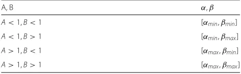
To maximizelog(y), iflog(A)is negative,αneeds to be as small as possible (sinceα > 0) elseαmust be as large as possible. Same applied toβ(Table 1).

Consider the case where we have a set of data points i.e. instead of constants A and B we have,

yi=uαiv β

i (18)

where i= 1 to N Our criterion is to chooseαandβso as to maximizey=n_i=1yii.e. maximize

N

i=1 yi=

_N

i=1 ui

α_N

i=1 vi

β

(19)

The RHS of (18) is similar in form to (16) and hence same rule can be applied i.e. IfN_i=1ui<1 thenα=αmin elseα = αmax. The term involvingβ can be minimized similarly and independently. The only remaining step is to determine the permissible ranges. Letbe the smallest value thatαandβcan take. Suppose in the above example,

N

i=1ui < 1 andiN=1vi >1. We know thatαshould be minimized andβshould be maximized. Sinceα+β <1, letα+β =1−δ, whereδis a small non-negative number. We then haveαmin=andβmax=1−δ−.

Results and discussion

As mentioned earlier, server and power/cooling costs form the biggest chunk of the total cost. These two inputs are considered for computing the values of the elasticities using 3D plots. However, the results obtained hold good for any number of inputs. It is also possi-ble to aggregate the inputs into two broad categories-operational expenditure and capital expenditure and use these as the two inputs in the proposed cost model. Operational expenditures include the recurring costs like power/cooling, server management etc; whereas capital expenditure includes initial investment such as new server cost, infrastructure costs etc.

Table 1Maximization of CD function for fixed A and B

A, B α,β

A<1,B<1 [αmin,βmin]

A<1,B>1 [αmin,βmax]

A>1,B<1 [αmax,βmin]

The data associated with data center costs from various sources have been accumulated and Cobb-Douglas func-tion is applied on varying elasticities to find the optimal solution for revenue of data center, and finally revenue maximization is demonstrated graphically. All simulation results have been generated by a computer system using Matlab.

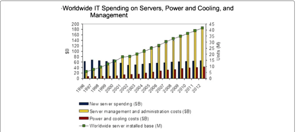
The approximate data from the Fig. 2 for two types of costs, namely server management/administrative cost and power/cooling cost are captured. The optimal elasticity of each input and maximum revenue for each year using Matlab code [Appendix 5] are obtained. The experiment has been conducted for the following three cases:

1) Increasing Returns to Scale 2) Constant Returns to Scale 3) Decreasing Returns to Scale

Case 1: increasing returns to scale Applying the constraints:

α+β >1

α >0

β >0

to the function: f =kxαyβ

Using fmincon function of matlab [Appendix 5], the val-ues of elasticities for which revenue is maximized for each year are obtained.

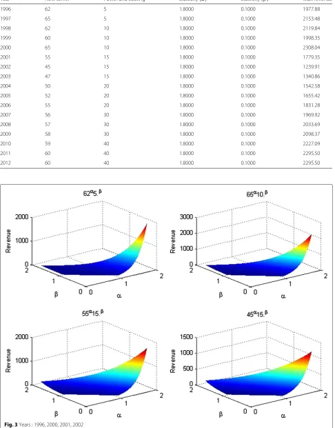
In Table 2, all units are in $B. The optimal revenue for all the years is obtained atα = 1.8 andβ = 0.1 Using these results, 3D-simulations are created and the corresponding graphs are obtained.

In Figs. 3 and 4, X axis represents output elasticity

α of new server expenditure, Y axis represents output

elasticity β of power/cooling cost and Z axis

repre-sents revenue. The graphs obtained depict the effects of Cobb-Douglas production function over worldwide IT spending in data center.It is observed that the graphs obtained are not concave graphs, which is shown math-ematically as well [Appendix 6]. It is prominent from

the graphs that revenues in the range of α around 1.8

and β around 0.1 give the optimal revenue for each

year.

It is seen from the data set that if new server cost is increased by 1 unit from year 2007($56B) to 2008($57B), the revenue changes by 63 units and when it is increased by 1 unit from year 2008($57B) to 2009($58B), the revenue changes by 64.68 units. This proves that marginal product of input (new server cost) increases in increasing returns to scale.

Case 2: constant returns to scale Applying the constraints:

α+β=1

α >0

β >0

to the function:f =kXαYβ

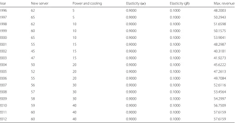
and using fmincon function of matlab [Appendix 5], the values of elacticities are obtained which maximize the revenue for each year, as shown in Table 3.

In Table 3, all units are in $B. The optimal

rev-enue for all years are obtained at α = 0.9 and

β = 0.1 Using these results, 3D-simulations are

cre-ated and the graphs of Constant Return to scale are obtained.

Table 2Simulation output for IRS

Year New server Power and cooling Elasticity_(α) Elasticity_(β) Max. revenue

1996 62 5 1.8000 0.1000 1977.88

1997 65 5 1.8000 0.1000 2153.48

1998 62 10 1.8000 0.1000 2119.84

1999 60 10 1.8000 0.1000 1998.35

2000 65 10 1.8000 0.1000 2308.04

2001 55 15 1.8000 0.1000 1779.35

2002 45 15 1.8000 0.1000 1239.91

2003 47 15 1.8000 0.1000 1340.86

2004 50 20 1.8000 0.1000 1542.58

2005 52 20 1.8000 0.1000 1655.42

2006 55 20 1.8000 0.1000 1831.28

2007 56 30 1.8000 0.1000 1969.92

2008 57 30 1.8000 0.1000 2033.69

2009 58 30 1.8000 0.1000 2098.37

2010 59 40 1.8000 0.1000 2227.09

2011 60 40 1.8000 0.1000 2295.50

2012 60 40 1.8000 0.1000 2295.50

Fig. 4Years : 2005, 2007, 2009, 2011

Table 3Simulation output for CRS

Year New server Power and cooling Elasticity(α) Elasticity(β) Max. revenue

1996 62 5 0.9000 0.1000 48.2003

1997 65 5 0.9000 0.1000 50.2943

1998 62 10 0.9000 0.1000 51.6598

1999 60 10 0.9000 0.1000 50.1575

2000 65 10 0.9000 0.1000 53.9041

2001 55 15 0.9000 0.1000 48.2987

2002 45 15 0.9000 0.1000 40.3181

2003 47 15 0.9000 0.1000 41.9273

2004 50 20 0.9000 0.1000 45.6222

2005 52 20 0.9000 0.1000 47.2613

2006 55 20 0.9000 0.1000 49.7084

2007 56 30 0.9000 0.1000 52.6116

2008 57 30 0.9000 0.1000 53.4564

2009 58 30 0.9000 0.1000 54.2997

2010 59 40 0.9000 0.1000 56.7509

2011 60 40 0.9000 0.1000 57.6159

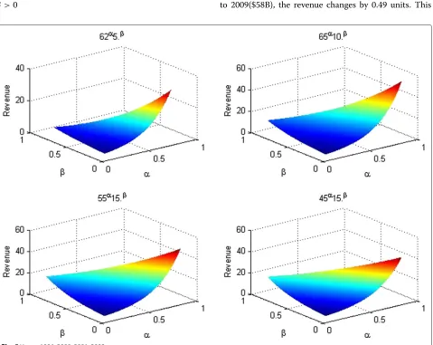
In Figs. 5 and 6, X axis represents output elasticity

α of new server expenditure, Y axis represents output

elasticityβ of power/cooling costs and Z axis represents revenue. The graphs obtained demonstrate the effects of Cobb-Douglas production function over worldwide IT spending in data center. It is observed that the graphs obtained are concave graphs, otherwise proved mathe-matically [Appendix 6]. The graphs reveal that revenues in the range ofαclose to 0.9 andβclose to 0.1 are optimal.

It is evident from the data set that if new server cost is increased by 1 unit from year 2007($56B) to 2008($57B), the revenue changes by 0.84 units. And when it is increased by 1 unit from year 2008($57B) to 2009($58B), the revenue changes by 0.84 units. This proves that marginal product of input (new server cost) is constant in constant returns to scale.

Case 3: decreasing returns to scale Applying the constraints:

α+β <1

α >0

β >0

to the function: f =kXαYβ

and using fmincon function of matlab [Appendix 5], the values of elacticities are obtained for which revenue is maximized for each year.

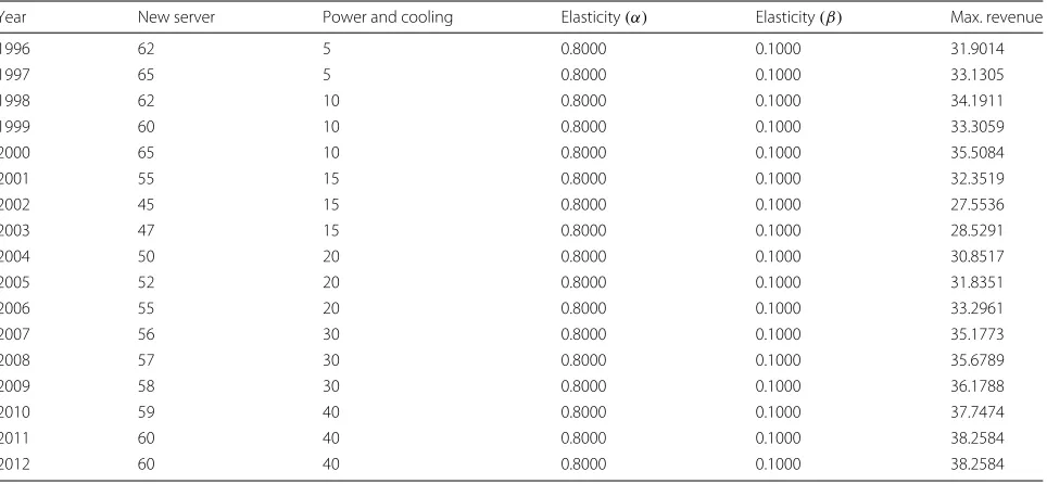
In Table 4, all units are in $B. The optimal revenue for all years are obtained atα=0.8 andβ =0.1.

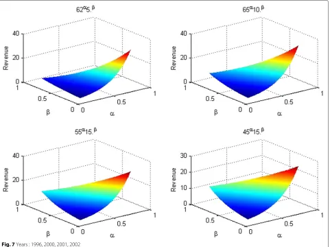
In Figs. 7 and 8, X axis represents output elastic-ity α of new server spending, Y axis represents output

elasticity β of power/cooling costs and Z axis

repre-sents revenue. The graphs obtained reflect the effects of Cobb-Douglas production function over worldwide IT spending in data center. We observe that the graphs obtained are concave graphs which has been proved math-ematically also [Appendix 6]. It is prominent from the graphs that revenues in the rangeα near 0.8 andβ near 0.1 give the optimal revenue for each year.

It can be seen from the data set that if new server cost is increased by 1 unit from year 2007($56B) to 2008($57B), the revenue changes by 0.50 units. And when it is increased by 1 unit from year 2008($57B) to 2009($58B), the revenue changes by 0.49 units. This

Fig. 6Years : 2005, 2007, 2009, 2011

Table 4Simulation output for DRS

Year New server Power and cooling Elasticity(α) Elasticity(β) Max. revenue

1996 62 5 0.8000 0.1000 31.9014

1997 65 5 0.8000 0.1000 33.1305

1998 62 10 0.8000 0.1000 34.1911

1999 60 10 0.8000 0.1000 33.3059

2000 65 10 0.8000 0.1000 35.5084

2001 55 15 0.8000 0.1000 32.3519

2002 45 15 0.8000 0.1000 27.5536

2003 47 15 0.8000 0.1000 28.5291

2004 50 20 0.8000 0.1000 30.8517

2005 52 20 0.8000 0.1000 31.8351

2006 55 20 0.8000 0.1000 33.2961

2007 56 30 0.8000 0.1000 35.1773

2008 57 30 0.8000 0.1000 35.6789

2009 58 30 0.8000 0.1000 36.1788

2010 59 40 0.8000 0.1000 37.7474

2011 60 40 0.8000 0.1000 38.2584

Fig. 7Years : 1996, 2000, 2001, 2002

proves that marginal product of input(new server cost) decreases in decreasing returns to scale.

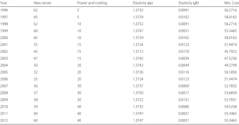
Gradient descent method has been applied on the same world wide IT spending dataset to find out optimal elastic-ities for cost minimization. As we have already proved that cost minimization can be achieved in increasing return to scale, the sum of the elasticities should be grater than 1. The initial values of the elasticities have been assumed as 1.2 and 0.7 whereas step size for each iteration has been considered as 0.001 (Table 5).

In the gradient descent calculation, we assumed the target revenue as $120B and unit cost of new server installation as 0.6.

Conclusion

In this paper, the proposed production model using Cobb-Douglas production function is used to quantify boundaries of the inputs (cost of servers, networking, infrastructure and power), for which the maximum rev-enue subject to the constraint that the total cost does not exceed a particular amount, is attained. These values

for the inputs are mentioned in Eqs. 2 through 5, and can be used to obtain the maximum revenue by substi-tuting in the production model. Similarly, the production model is also used to obtain the minimum total cost sub-ject to a certain amount of production (output) that has to be achieved. This value of total minimum cost can be computed using Eq. 9. Further, the inputs contributing to the maximum profit are deduced, as evident from Eqs. 11 through 14. Computation of revenue function using the production model, a subsequent operation, becomes straight forward enough.

Fig. 8Years : 2005, 2007, 2009, 2011

Table 5Gradient descent output for costminimization

Year New server Power and cooling Elasticity(α) Elasticity(β) Min. Cost

1996 62 5 1.3732 0.0091 56.2716

1997 65 5 1.3729 0.0102 58.0163

1998 62 10 1.3732 0.0091 56.2716

1999 60 10 1.3747 0.0031 55.3465

2000 65 10 1.3729 0.0102 58.0163

2001 55 15 1.3724 0.0123 51.9474

2002 45 15 1.3712 0.0170 45.7922

2003 47 15 1.3745 0.0039 47.5236

2004 50 20 1.3742 0.0049 49.2799

2005 52 20 1.3726 0.0116 50.1856

2006 55 20 1.3724 0.0123 51.9474

2007 56 30 1.3737 0.0069 52.7832

2008 57 30 1.3750 0.0017 53.6839

2009 58 30 1.3722 0.0131 53.7031

2010 59 40 1.3735 0.0080 54.5258

2011 60 40 1.3747 0.0031 55.3465

Further, it is also established that the cost minimization with production constraint will be achieved at the phase of increasing returns to scale (IRS) of the enterprise.

α+β+γ +δ >1

and profit maximization will take place at the phase of decreasing returns to scale (DRS).

α+β+γ +δ <1

Finally, this paper shows simulations for a given data set, and it is seen that for every phase (IRS, CRS or DRS), there exists a common optimal value of elasticities (α andβ) for annual data, which maximizes the revenue. It is also observed from the 3D graphs that the production function is concave for constant and decreasing returns to scale this signifies the enterprise will definitely reach a point where its profit will be maximum for a particular invest-ment. Whereas, it is neither concave or convex for the increasing return to scale, which signifies that the enter-prise will reach a point where it is able to minimize the investments made and achieve a target output. Therefore, it can be seen from these 3D graphs and optimal output elasticities that the production model proposed agrees with the current practices in industry.

It has also been established that the behavior of the marginal product of an input depends on the phase of the enterprise. It will rise during increasing returns to scale phase, stay stable for constant returns phase and fall for the last phase of decreasing returns to scale.

An enterprise investing in the data center may be will-ing to suffer a decrease in production by 10 % or less, at the cost of a major decrement in total investment made on the inputs. This compromise with the yearly pro-duction can increase the overall profit of the enterprise drastically. This result needs confirmation by analyzing the different values of inputs for a deviation of revenue ranging from 0–10 %. For example, consider the invest-ments made in the year 2009, (Table 1). The maximum revenue is $36.1788B. If the enterprise decides to decrease investment on servers to $55B and on power & cooling to $28B, the revenue decreases to $34.4354B. Therefore, the output decreases by $1.7434B (that is 4.8 %), but at the same time, the cost of input decreases by a total of $2B. Thus, overall profit increases. Tables 2 and 3 fortify our observation further. Table 2 shows that an increase in the cost of server while keeping power and cooling costs did not impact the revenue. In fact, the revenue increased. Table 3 demonstrates the fact that a decrease in server cost coupled with a twofold increase in power plus cooling cost did not affect revenue in a negative way. Gradient descent ensures that cost is achieved to be minimal by manipulat-ing the elasticities and the increase in revenue is observed accordingly.

The above results are obtained taking into considera-tion two major cost factors, servers, and power. These results can be extended to any cost model with more number of inputs. In spite of its application in various fields, Cobb-Douglas production function has the follow-ing

limitations-• It does not allow identification of the nature of technological progress [35].

• It may suffer from curvature violation and sometimes it requires estimation of many parameters [36].

In the context of the our proposed model, nature of technological progress is not very important as we have not instrumented this in our model. Curvature violation is a major issue, in case of flexible functional form. We expect the global curvature conditions to be consistent with economic theory when estimations of cost, profit, revenue are required from a functional form. Along with that, the task of maintaining the flexibility of functional form is also necessary. Translog function is a generalized form of Cobb-Douglas function, a flexible functional form providing second order approximation. Both the Cobb-Douglas and Translog functions are linear in parameters and can be estimated using least squares methods. It is possible to impose restrictions on the parameters (homo-geneity conditions). C-D functions are simplistic, assumes all firms have same production elasticities and that sub-sitution elasticities equal 1. Translog function, which is a generalization of Cobb-Douglas, suffers from curvature violation. But we have not implemented Translog function in our model. Multiple test cases run on several differ-ent values don’t indicate any curvature violation (cf. Fig. numbers 1–5).

General Notes on Curvature violations (Change of sign):

- Translog function is very commonly used.

- It is a generalization of the Cobb-Douglas function. - It is a flexible functional form providing a second

order approximation.

- Cobb-Douglas and Translog functions are linear in parameters and can be estimated using least squares methods.

lnqi=b0+b1lnx1i+b2lnx2i+vi+ui

Translog:

lnqi = b0 + b1lnx1i + b2lnx2i + 0.5b11(lnx1i)2 + 0.5b22(lnx2i)2+b12lnx1ilnx2i+vi+ui

The disadvantages of Translog function are listed below:

• It is more difficult to interpret.

• Translog function requires many parameters for estimation.

The curvature violation is not evident for Cobb-Douglas in the case of CRS (Constant return to scale) and DRS (Decreasing return to scale). It may arise when we con-sider IRS (Increasing return to scale). This IRS curvature violation issue can be tackled using Monte Carlo simula-tion. In theory, it’s a technical possibility but the authors have not encountered in this study. In fact, Translog production functions requires estimation of many param-eters: K+3+K(K+1)/2 and may suffer from curvature violations. On the other hand, Cobb-Douglas, having lin-ear parameters (in logs) estimated or simulated at par with this assumption, and empirically speaking, we do not see too many curvature violations (on higher orders) for such production/cost functions. If there are, it sometimes arises due to added local (meaning industry-specific, product specific, as opposed to global meaning universal-ized) restrictions, which we haven’t instrumented in our structure and need not be concerned about. In cases of stochastic frontier analysis estimates with Translog (and therefore quadratic forms) the curvature violation is much more feasible than a Cobb Douglas production function. Considering all these points, Cobb-Douglas is a more suit-able option in comparison to Translog as a foundation of our mathematical model.

This production model obtained from Cobb-Douglas function might also prove to be helpful in forecasting the revenue of a cloud data center. An enterprise planning to set-up a data center may want to know the approximate revenue for a particular capital expenditure on the inputs. The future revenue estimates may be determined by using this production function [Appendix 7].

Chandrakant et al in their paper Cost Model for Plan-ning, Development and Operation of a Data Center have considered four key cost components (space, power, cool-ing, operation) in total cost calculation. Individual cost component has been discussed in details based on their dependency on different parameters such as amortiza-tion cost, maintenance cost and the influence on the total cost. These apart, other cost factors (Licensing cost, Per-sonnel cost, Operation cost) have also been incorporated in the cost model. In contrast, our proposed model is not dependent on the number of cost components. The Cobb-Douglas model can be expanded as it can accom-modate any number of cost factors. Our model not only highlighted cost optimization but also had shown how to achieve profit maximization, revenue maximization. Using real world data set we have established the effi-ciency of our suggested mathematical model. Jim Gao, in his Machine Learning Applications for Data Center Optimization paper, rigorously used machine learning application to model data center performance and energy efficiency. Various challenges related to data center have been discussed and neural network has been implemented to build the mathematical framework. Energy efficiency

is the prime objective of the optimization model and the performance of the model is limited by the quality and quantity of data inputs like any other machine learning applications. In contrast, our model is independent on the training set and methods of training the machine.

Paul J.J. Welfens in his paper ‘A Quasi-Cobb Douglas Production Function with Sectoral Progress: Theory and Application to the New Economy’ proposed a new mathematical model based on Cobb-Douglas function, which can shed light on process innovation dynamics – this includes a distinction between Harrod neutrality and Solow neutrality of technological progress. The model is an example of endogenous growth approach in which one can study different types of technological progress. It is assumed that Solow type technological progress was determined by ICT capital only. The model has been developed based on two sector production function, where the sectoral Solow progress depends on the hybrid sectoral capital intensity.

Y = [B(K/L)K]β[K]β[AL]1−β−β (20)

whereK=ICT -capitalK=non-ICT capital. K denotes capital and L denotes labor. According to the assumption, sectoral Solow progress B in the sector using ICT capital is associated with K’/L (hybrid sectoral capital intensity). The parameter B(K’/L) implies the ICT sector, character-ized by capital-saving technological progress which can be found in various fields such as computer chip (Moore’s law which says that the power of computing chip will dou-ble within 3 or more recently 2 years) and fiber optical cables. The information and communication technology (ICT) and other few factors are the key reasons behind the technological progress.

Additional remarks & future work

Technological progress

AWS and other data center providers are constantly improving the technology and define the cost of servers as the principle component in the revenue model. For example, AWS [31] spends approximately 57 % of their budget towards servers and constantly improvise in the procurement pattern of three major types of servers. The model used by the authors need to look at such situation i.e include three different input variables for the costs of three different types of servers. In essence, a whole body of future work may include incorporating a lot of input parameters and subject the Cobb Douglas model to mul-tiple levels of the same parameter, namely power cost. This leads to a possibility of interesting analytical exercise, coupled with a full factorial design of an experiment.

Experimental design

variables on the revenue in terms of percentage contribu-tion of each variable. An efficient, discrete factorial design could be implemented to study the effects and changes in all relevant parameters regarding revenue. Revenue may be modeled as y, dependent on a constant (market force) and a bunch of input variables, quantitative or categor-ical in nature. The road-map to design a proper set of experiments for simulation involves the following:

• Develop a model best suited for the data obtained.

• Isolate measurement errors and gauge confidence intervals for model parameters.

• Check the adequacy of the model.

Response variable is the outcome, e.g. revenue output due to factors such as cost, man-hours and the levels of those factors. The primary and secondary factors as well as replication patterns need to be ascertained such that the impact of variation among the entities is minimized. Interaction among the factors need not be ignored. A full factorial design with the number of experiments equal to

_k

i=1niwould capture all interactions and explain varia-tions due to technological progress, the authors believe. Here, n denotes the number of factors and k stands for different levels each factor may have [37].

Appendix 1

The Lagrangian function for the optimization problem is:

L=y−λ(w1S+w2I+w3P+w4N−m)

L=kSαIβPγNδ−λ(w1S+w2I+w3P+w4N−m)

The first order conditions are:

∂L

∂S =kαS

α−1_Iβ_Pγ_Nδ_−w

1λ=0 (21)

∂L

∂I =kβS

α_Iβ−1_Pγ_Nδ_−w

2λ=0 (22)

∂L

∂P =kγS

α_Iβ_Pγ−1_Nδ_−w

3λ=0 (23)

∂L

∂N =kδS

α_Iβ_Pγ_Nδ−1_−w

4λ=0 (24)

∂L

∂λ = −(w1S+w2I+w3P+w4N−m)=0 (25)

Dividing (22), (23), (24) by (21),

I= β

α

w1 w2 S

P= γ

α

w1 w3 S

N= δ

α

w1 w4 S

Substituting these values in (25),

S= mα w1(

1+β+γ +δ) (26)

Similarly,

I= mβ w2(

1+α+γ +δ) (27)

P= mγ w3(

1+α+β+δ) (28)

N= mδ w4(

1+α+β+γ ) (29)

Appendix 2

The Lagrangian function for the optimization problem is:

L=w1S+w2I+w3P+w4N−λ(f(S,I,P,N)−ytar) (30)

The First order conditions are;

∂L

∂S =w1−λkαS

α−1_Iβ_Pγ_Nδ_{=0 (31)}

∂L

∂I =w2−λkβS

α_Iβ−1_Pγ_Nδ_{=0 (32)}

∂L

∂P =w3−λkγS

α_Iβ_Pγ−1_Nδ_{=0 (33)}

∂L

∂N =w4−λkδS

α_Iβ_Pγ_Nδ−1_{=0 (34)}

∂L

∂λ =kSαIβPγNδ−ytar=0 (35)

Dividing Eqs. (32), (33) and (34) by (31); we obtain

I= β

α

w1 w2 S

P= γ

α

w1 w3 S

N= δ

α

w1 w4 S

Substituting these values in Eq. (35); we obtain

⇒ytar=kSα β α w1 w2 S β_γ α w1 w3 S γ_δ α w1 w4 S δ

⇒ytar=kSα+β+γ+δα−β−γ−δββγγδδwβ1+γ+δw2−βw−3γw−4δ

⇒Sα+β+γ+δ =k−1αβ+γ+δβ−βγ−γδ−δw₁−β−γ−δw₂βwγ₃wδ₄ytar

⇒S=k−1αβ+γ+δβ−βγ−γδ−δw−₁β−γ−δwβ₂wγ₃wδ₄ytar 1

α+β+γ+δ

⇒w1S=

k−1αβ+γ+δβ−βγ−γδ−δwα₁wβ₂wγ₃wδ₄ytar 1

α+β+γ+δ

Similarly,

w2I=

k−1α−αββ+γ+δγ−γδ−δwα₁wβ₂wγ₃wδ₄ytar

1 α+β+γ+δ

(37)

w3P=

k−1α−αβ−βγβ+γ+δδ−δwα₁wβ₂wγ₃wδ₄ytar

1 α+β+γ+δ

(38)

w4N=

k−1α−αβ−βγ−γδβ+γ+δwα₁wβ₂wγ₃wδ₄ytar

1 α+β+γ+δ

(39)

The cost for producing ytar units in cheapest way is c, where

c=w1S+w2I+w3P+w4N (40)

From (31), (32), (33) and (34), Eq. (35) can be written as;

c=Q

wα₁wβ₂wγ₃wδ₄

1 α+β+γ+δ y 1 α+β+γ+δ tar (41) where,

Q=kα+β−+1γ+δ

_αβ+γ+δ ββ _+γγ_+δδ + βα+γ+δ αα_+γγ _+δδ +_ααγ₊α+_ββ_β+₊δ _δδ + _αα+δα+_ββ_β+₊γ_γγ 1 α+β+γ+δ

Cavg= C ytar =

Q

wα₁wβ₂wγ₃wδ₄

1 α+β+γ+δ

y

1 α+β+γ+δ−1 tar

Appendix 3

The conditions for optimization:

pαkSα−1IβPγNδ=w1 (42)

pβkSαIβ−1PγNδ=w2 (43)

pγkSαIβPγ−1Nδ=w3 (44)

pδkSαIβPγNδ−1=w4 (45)

Multiplying these equations with S, I, P and N,

respectively-pαkSαIβPγNδ=w1S⇒pαy=w1S (46)

pβkSαIβPγNδ=w2I⇒pβy=w2I (47)

pγkSαIβPγNδ=w3P⇒pγy=w3P (48)

pδkSαIβPγNδ=w4N⇒pδy=w4N (49)

Dividing Eqs. (47), (48) and (49) by (46) following equations are obtained:

I= β

α

w1 w2

S (50)

P= γ

α

w1 w3

S (51)

N= δ

α

w1 w4

S (52)

Substituting these values of I, P and N in (42), we get

pαkSα−1IβPγNδ=w1

⇒pαkSα−1

_β

α

w1

w2S β_γ

α

w1

w3S γ_δ

α

w1

w4S δ

=w1

⇒pkSα+β+γ+δ−1ββγγδδw₁β+γ+δ−1w−₂βw₃−γw−₄δ=1

⇒S=pkα1−(β+γ+δ)ββγγδδw₁β+γ+δ−1w₂−βw−₃γw−₄δ 1 1−(α+β+γ+δ)

(53)

Performing similar calculations the following values of I, P and N are obtained:

I=pkααβ1−(α+γ+δ)γγδδw₁−αwα₂+γ+δ−1w−₃γw−₄δ

1 1−(α+β+γ+δ)

(54)

P=pkααββγ1−(α+β+δ)δδw₁−αw₂−βw₃α+β+δ−1w−₄δ

1 1−(α+β+γ+δ)

(55)

N=

pkααββγγδ1−(α+β+γ )w₁−αw−₂βw₃−γwα₄+β+γ−1

1

1−(α+β+γ+δ)

(56)

These values of S, I, P and N are the profit maximizing data center’s demand for inputs, as a function of the prices of all the inputs, and of the price of output. Substituting values of S, I, P and N into Eq. (1), we get

y=kpα+β+γ+δααββγγδδw−₁αw−₂βw−₃γw−₄δ

1 1−(α+β+γ+δ)

(57)

Appendix 4

Consider the following production function:

y= n

i=1 kxαi

i

To prove:

n

i=1