R E S E A R C H
Open Access
Efficient resource provisioning for
elastic Cloud services based on machine
learning techniques
Rafael Moreno-Vozmediano
1*, Rubén S. Montero
1, Eduardo Huedo
1and Ignacio M. Llorente
1,2Abstract
Automated resource provisioning techniques enable the implementation of elastic services, by adapting the available resources to the service demand. This is essential for reducing power consumption and guaranteeing QoS and SLA fulfillment, especially for those services with strict QoS requirements in terms of latency or response time, such as web servers with high traffic load, data stream processing, or real-time big data analytics. Elasticity is often implemented in cloud platforms and virtualized data-centers by means of auto-scaling mechanisms. These make automated resource provisioning decisions based on the value of specific infrastructure and/or service performance metrics. This paper presents and evaluates a novel predictive auto-scaling mechanism based on machine learning techniques for time series forecasting and queuing theory. The new mechanism aims to accurately predict the processing load of a distributed server and estimate the appropriate number of resources that must be provisioned in order to optimize the service response time and fulfill the SLA contracted by the user, while attenuating resource over-provisioning in order to reduce energy consumption and infrastructure costs. The results show that the proposed model obtains a better forecasting accuracy than other classical models, and makes a resource allocation closer to the optimal case.
Keywords: Cloud computing, Elasticity, Auto-scaling, Machine learning
Introduction
Service elasticity is a common feature offered by many cloud platforms and virtualized data-centers. This can be defined as the ability to adapt the system to work-load changes, by autonomously provisioning and depro-visioning resources, so that at each point in time, the available resources match the current service demand as closely as possible [1]. The advantages of using service elasticity mechanisms are twofold. On the one hand, it provides Quality of Service (QoS) to the users, which can be expressed using different service metrics, such as response time, throughput (e.g., requests/s), service avail-ability, and so on, depending on the service type. The QoS levels agreed between the service provider and user are defined by means of Service Level Agreements (SLAs), in such a way that service level failures can result in cost penalties for the service provider and a potential loss of
*Correspondence:[email protected]
1Computer Science School, Complutense University, 28040 Madrid, Spain Full list of author information is available at the end of the article
clients. On the other hand, service elasticity enables power consumption to be reduced, by avoiding resource over-provisioning. Over-provisioning is a typical and simple solution adopted by many service providers to satisfy peak demand periods and guarantee QoS during the service lifetime. However, this results in a waste of resources that remain idle most of the time, with the consequent super-fluous power consumption and CO2 emissions. The use of service elasticity mechanisms enables a reduction in the number of resources needed to implement the service and, along with other efficient techniques for server con-solidation, virtual machine allocation, and virtual machine migration, it can lead to important energy savings for the datacenter or cloud provider [2–4].
Cloud providers often implement elasticity by using auto-scaling techniques [5]. These make automated scal-ing decisions based on the value of specific perfor-mance metrics, such as hardware metrics (e.g. CPU or memory usage) or service metrics (e.g., queue length, service throughput, response time, etc.). Auto-scaling mechanisms can be classified as reactive and proactive.
Reactive mechanisms are continuously monitoring the system, and trigger a particular scaling action when a spe-cific condition is met (e.g., provisioning or removing a given number of resources when a particular metric is higher or lower than a particular threshold). The main problem with reactive mechanisms is that the reaction time (time elapsed from the detection of the trigger con-dition until the resources are ready for use) can be insuffi-cient to avoid the overloading of the system; furthermore, these mechanisms can cause system instability due to the continuous fluctuation of allocated resources. In contrast, proactive (or predictive) mechanisms try to predict the amount of resources needed during the next time period, based on statistical or mathematical models of observed workloads and system metrics. Although most existing cloud platforms and providers use reactive models, there is a great deal of research on predictive models based on time series analysis, queuing theory, reinforcement learning, or control theory, among other aspects [6].
Time series analysis has been widely used to implement auto-scaling mechanisms for applications that exhibit some kind of temporal patterns. Most of these proposals (e.g., [7–10]) use linear statistical methods for time-series forecasting, mainly based on Box and Jenkins [11] autore-gressive models (e.g., AR, ARMA, ARIMA, or ARMAX) for predicting service metrics (e.g., the server load) from historical observations. However, as these service met-rics can exhibit non-linear patterns, some key features of the input data may not be properly captured by these linear models. Some other studies [12,13] use nonlinear regression models based on neural networks. The main inconvenience of these methods is the difficulty of design-ing the network topology of the neural network so that it is efficient, in addition to the training of algorithms, which can be slow, and can get stuck in local minima. Regarding the limitations of these methods, in this work we pro-pose a novel predictive auto-scaling mechanism based on Machine Learning (ML) techniques for time series fore-casting, in particular, the Support Vector Machine (SVM) regression technique [14,15], combined with queue the-ory for modeling the system performance. The main advantage of the SVM regression model is that it fits well to input data with both linear and nonlinear patterns, and always reaches a unique global solution, with reasonable training times.
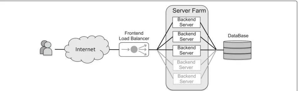
This auto-scaling mechanism is aimed at achieving an accurate prediction of the load of an elastic cloud ser-vice (e.g., a web server cluster or data stream process-ing server), as shown in Fig. 1. This figure represents a typical elastic web server cluster, consisting on a ser-vice front-end, acting as load balancer, and a variable number of backend servers that process users requests. The auto-scaling mechanisms should allow the system to dynamically adapt to workload changes, by autonomously
provisioning and de-provisioning resources (i.e., back-end servers), so that at each point in time, the available resources match the current service demand as closely as possible. More specifically, we propose the use of SVM regression to predict the server’s processing load (requests/s) based on historical observations, and then we model the performance of the system using a M/M/c
queue model [16] to determine the optimal number of
resources (backend servers) that must be allocated to sat-isfy the predicted server demand and fulfill the SLAs (e.g., response time), while trying to avoid excessive resource over-provisioning, thereby reducing energy consumption and infrastructure costs.
We have compared the proposed ML-based auto-scaling mechanism with other classical forecasting mech-anisms, including prediction based on last value, the mov-ing average model, and the linear regression model. Our results show that the SVM regression model displays bet-ter forecasting accuracy than the classical models, and facilitates better resource allocation, closer to the optimal case.
The main contributions of this paper are the following: • A novel auto-scaling method based on ML
techniques aimed at optimizing the service latency (response time) and reducing over-provisioning of elastic cloud services.
• A SVM regression model for predicting the server’s processing load.
• Optimal selection of SVM regression model parameters based on an analytical method.
• A queue-based performance model for determining the number of resources that must be provisioned based on the predicted load.
• An evaluation using load data from a real server.
This paper is organized as follows:Related worksection includes the related work on dynamic resource provi-sioning mechanisms for providing service elasticity. The ML-based forecasting techniques and the performance
model are described in Time series forecasting using
machine learning techniques section and Performance model section. Evaluation section evaluates the accu-racy of ML-based forecasting methods and the result-ing resource allocation decisions. Finally,Conclusion and Future Worksection summarizes the main conclusions of the paper.
Related work
Fig. 1Elastic cloud service. This figure represents a typical elastic web server cluster, consisting on a service front-end, acting as load balancer, and a variable number of backend servers that process users requests. The cloud auto-scaling mechanisms allow to dynamically adapt the system to workload changes, by autonomously provisioning and deprovisioning resources (i.e., back-end servers), so that at each point in time, the available resources match the current service demand as closely as possible
mentioned above, there are many other proposals and realizations of auto-scaling strategies based on many dif-ferent mechanisms, such as threshold-based policies, con-trol theory, reinforcement learning, or queuing theory, among others.
Threshold-based mechanisms are reactive auto-scaling algorithms implemented by various cloud providers and platforms (e.g. Amazon EC2, RightScale, and OpenNebula [27]) that enable users to define up and scaling-down policies or rules based on different metrics. These rules are defined in terms of specific upper and/or lower thresholds for the selected metric, so that if the metric is over (or under) the established threshold for a given time interval, it triggers a scaling action by adding (or removing) a given amount of resources from the infras-tructure. Some research works have proposed certain improvements to the basic threshold-based mechanisms, for example Hasan et al. [28] propose the use of auto-scaling policies based on four threshold values, allowing finer autoscaling decisions than if only two thresholds are used; Chieu et al. [29] suggest an extension of the RightScale method based on the number of active ses-sions, so that to trigger the provisioning of a new instance, the number of active sessions in all instances must exceed a certain threshold.
There are several auto-scaling mechanism proposals based on the concepts of control theory. They usually implement a controller that is responsible for maintain-ing the output of the system (e.g., the throughput or the latency of the system) at a specific level, by adjusting the control input (e.g., the number of allocated resources). Most control-based systems are reactive mechanisms,
for example Lim et al. [30] propose extending the
cloud platform with an external feedback controller that enable users to automate the resource provisioning, and introduce the concept of proportional thresholding, a new control policy that takes into account the
coarse-grained actuators provided by resource providers; and Padala et al. [31] also use a feedback control system to dynamically allocate resources to applications running on virtualized infrastructure. This is based on a MIMO (multi-input, multi-output) resource controller that deter-mines appropriate allocations of multiple resources to achieve application-level SLOs. However, there are also some proposals related to proactive control-based auto-scaling mechanisms; for example, Roy et al. [9] propose a predictive solution based on a look-ahead optimiza-tion controller. This iteratively solves an optimizaoptimiza-tion problem over a predefined horizon, taking into account current and future constraints, by combining the control-based solution with a time series mechanism, control-based on autoregressive moving average forecasting, to pre-dict the workload of the application. A major draw-back of control theory approaches is the difficulty of selecting the correct gain parameters for the model, as these may cause system instability if they are not adequate.
initialization for the early stages of learning, convergence speedup techniques to reduce the error and improve learning time, and performance model change detection. Other studies have also addressed these problems, for example, Tesauro et al. [33] propose a hybrid approach than combines the strengths of both RL and queuing mod-els, in which RL trains offline on data collected while a queuing model policy controls the system, in order to avoid suffering potentially poor performance in live online training; and Barrett et al. [34] use a RL algorithm known as Q-learning to implement optimal scaling policies in cloud environments, and propose a parallel version of the Q-learning algorithm to reduce the execution time.
Queueing theory can also be used to implement autoscaling mechanisms, by using a queue model of the system and making decisions based on different optimiza-tion parameters, such as average queue length, average queue time, or average response time. For example, Salah
et al. [35] propose a Markov chain analytical model,
based on a finite queueing system, to provide elastic-ity for cloud-hosted applications; and Kaur and Chana [36] propose a QoS-aware resource elasticity framework, modeled as a closed-form queuing network model, which implements a proactive technique for estimating the elas-ticity level of machines required at each tier of the application.
Queuing theory has also been combined with other techniques, such as time-series prediction [7, 8], to improve the quality of auto-scaling mechanisms. This combined approach has also been utilized in this work: we first use an efficient time series model, based on SVM regression, to predict the load of a distributed server, and, based on these predictions, we propose a queue performance model to make a near-optimal resource provision for the server. This auto-scaling approach is well-suited to applications that exhibit either linear or non-linear temporal patterns, it is easy to implement as it does not require the development of complex con-trollers or decision making agents, and it requires a reasonably short execution time to make auto-scaling decisions.
Time series forecasting using machine learning techniques
The auto-scaling method proposed in this work is based on forecasting the load of a distributed server, so that we can estimate the optimal number of resources that must be allocated to satisfy the predicted demand in order to optimize the service response time and reduce over-provisioning. The forecasting method uses time series modeling, i.e., based on past observations of the server load we develop an appropriate model to describe the structure of the series, and we use this model to predict future values.
Time-series analysis is a broad discipline that has been applied to many different fields, such as business, eco-nomics, finance, science, and engineering. There are many different methods for time-series modeling and forecast-ing, although some of the most popular are the statistical methods developed by Box and Jenkins [11], such as the ARMA and ARIMA models. The main advantage of these models is their flexibility and simplicity when represent-ing several varieties of time series, as these characteristics make them quick and easy to use. They do, however, present an important limitation due to their linear behav-ior; this makes them inadequate in many practical situ-ations. More recently, different methods for time series forecasting based on ML techniques have been proposed [37, 38], including Artificial Neural Networks (ANNs)
[39, 40] and Support Vector Machine (SVM) methods
[41, 42], which have inherent nonlinear-modeling capa-bilities. ANN methods are inspired by biological systems, and try to learn from experience to provide generalized results based on their knowledge; ANNs are data-driven and self-adaptive methods that do not make a priori assumptions about the models or data distributions. The main drawback of ANN methods is that they can suffer from multiple local minima, and do not provide a unique global solution. In contrast, SVMs are nonlinear and used for classification, regression, and time-series prediction based on the structural risk minimization principle. SVMs map the input data into a high-dimensional space using nonlinear mapping, and then perform a linear regression of this space. The main advantage of SVM is that the solu-tion obtained is always unique and globally optimal. In this work we use the SVM method for time series forecasting.
Time series training data
A time series is a set of time dependent observations of one or more variables of a system. For example, for a dis-tributed service, such as a web server cluster or a data stream processing server, we take the values of the hourly average system load (measured in requests/s) forNtime periods, resulting in a time series s = {s1,s1,. . .,sN}, si ∈ R,∀i ∈ {1,N}. The goal of the forecasting method is to predict the value of this variable for the subsequent time periods, i.e., sN+1,sN+2,. . .; this is known as the forecasting horizon.
Before applying the SVM technique for time series forecasting, the observed data must be modeled as input/output pairs, called training sets, by splitting the time series into windows of lagged variables of
size T, i.e., for each training input window xm =
{sm−T−1,. . .,sm−2,sm−1}, the corresponding training
out-put isym=sm.
• The[M×T]input training matrix: X= ⎡ ⎢ ⎢ ⎢ ⎣
sN−1 sN−2 . . . sN−T−1 sN−2 sN−3 . . . sN−T−2
..
. ... . .. ... sT sT−1 . . . s1
⎤ ⎥ ⎥ ⎥ ⎦
• The[M×1]output training vector:
Y= ⎡ ⎢ ⎢ ⎢ ⎣ sN sN−1
.. . sT+1
⎤ ⎥ ⎥ ⎥ ⎦
The support vector regression model
A detailed description of SVM theory and its applica-tions [41,43–46] is beyond the scope of this paper, so this section highlights the main elements of the SVM model for time series forecasting used in this work, which is based on the sequential minimal optimization algorithm for SVM regression [14,15].
SVM is a machine learning technique that learns from nonlinear input training data using a linear learner. For this purpose, the SVM regression maps the input data into a high-dimensional feature space via nonlinear mapping using akernel function. Then, a linear regression model is used to regress in the new feature space. In the case of time series forecasting, where we have a training set of M input/output pairs(xm,ym)m=1...M, the SVM regres-sion can approximate the value of the time series at timet, using the following function:
ˆ yt=b+
M
m=1
wm×K(xt,xm) (1)
wherebis a constant (bias term);wmare the weight factors (W = {w1,w2,. . .,wM}is the weight vector);xtis the time series data window at timet; andKis the kernel function. The goal of the SVM algorithm is to find the optimal weight vector,W, that minimizes the regularized risk,Rreg, defined as follows:
Rreg= 1 2
M
m=1 w2m+C
M
m=1
L(ym,yˆm) (2)
The first term of the risk function enforces flatness in the feature space, by penalizing the model complexity. The second term is the Vapnik-insensitive loss function [46], which measures the empirical error between the model estimation (ˆym) and the real data(ym), penalizing those errors larger than±, and is defined as follows:
L ym,yˆm
=
|ym− ˆym| − if|ym− ˆym|>
0, otherwise (3)
Constant C in Eq. 2 (with C > 0) modulates the
trade-off between the model flatness and the amount of
tolerated deviations larger than. The optimal values of
bothandCare data dependent, and have to be chosen
by the user. However, there are some analytical methods that can help to select these parameters [47].
To cope with errors larger than , the slack variables, ξ andξ∗can be introduced into the model. These repre-sent the functional distance of two possible, but mutually exclusive samples. So, the expression of regularized risk to be minimized in Eq.2can therefore be reformulated as follows:
Rreg= 1 2
M
m=1 w2m+C
M
m=1
(ξm+ξ∗ m)
subject to ⎧ ⎨ ⎩
ym− ˆym−b≤+ξm∗ ˆ
ym+b−ym≤+ξm ξm,ξm∗ ≥0
(4)
The minimization of Eq. 4 is a standard problem of
minimization with constraints, which can be solved by applying Lagrangian theory. Then, the weight vector,W, can be obtained from Lagrange multipliers,αm andα∗m, which are associated with a specific training point:
wm=αm−α∗m,∀m∈ {1,M}
subject to M
m=1(αm−αm∗)=0 αm,αm∗ ∈[ 0,C]
(5)
Based on the Karush-Kuhn-Tucker conditions [44], only
a reduced number of coefficients αm and αm∗ will be
non-zero, and the training points associated with these parameters refer to the model support vectors.
Kernel functions
The kernel function [15, 48] transforms the nonlinear input space into a high-dimensional feature space. In this space, the problem can be solved as a linear prob-lem. Some of the most common kernel functions are the following:
• Polynomial kernel. One of the most common polynomial kernels is:
K x,x= x·x+1p (6)
wherex·xis the dot product of feature vectorsx andx, andp∈Nis the exponent of the kernel, chosen by the user.
• Normalized polynomial kernel. The normalized polynomial kernel is a variant of the polynomial kernel, which can defined as:
K x,x= x·x +1p
||x||||x|| (7)
• RBF kernel. The radial basis function (RBF) or Gaussian kernel is defined as:
K x,x=e−γ||x−x||2 (8)
where||x−x||2represent the Euclidean distance between feature vectorsx andx, andγ ∈Ris a user-defined parameter.
In the literature we can find many other kernel func-tions, such as the Fourier kernel [46], the Pearson VII function-based kernel (PUK) [49], and the multilayer per-ceptron kernel [50], among others. However, in this work we will use the above-defined basic kernels.
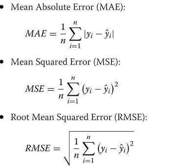
Forecast accuracy measures
Different error measures can be used to evaluate the accu-racy of the forecasting models. Some of the most common error measures are the following:
• Mean Absolute Error (MAE):
MAE= 1
n n
i=1
|yi− ˆyi| (9)
• Mean Squared Error (MSE):
MSE= 1
n n
i=1 yi− ˆyi
2
(10)
• Root Mean Squared Error (RMSE):
RMSE=
1
n n
i=1 yi− ˆyi
2
(11)
If the previous accuracy measures are applied to the training data set of the time series, they provide an esti-mation of how the forecasting model fits these historical data, i.e., they measure the expected or estimated predic-tion error of the forecasting model. On the other hand, if we apply these accuracy measures to the forecast data within the forecasting horizon, assuming we know the real
values of the time series for this period, we obtain the real prediction error made by the forecasting model.
Performance model
The time series forecasting method described in the pre-vious section enables load predictions to be made for an elastic cloud service based on historical observations. The next challenge to address is the development of an accurate performance model, based on these predictions, to decide the optimal number of resources (i.e., backend servers) that must be allocated to the system, in order to fulfill the SLAs contracted with the users. The system performance model proposed in this work is based on queuing theory.
We assume that the server, as shown in Fig.1, has a sin-gle front-end entry point for all the users, and the various client requests are distributed to different parallel backend servers using a load balancer. This distributed server can be modeled as a M/M/c queue [16], as shown in Fig.2.
The M/M/c queue model is based on the following parameters:
• c is the number of parallel servers in the system.
• λis thearrival rate, i.e., the average number of requests that reach the system per time unit, modeled as a Poisson distribution.
• μis theservice rate, i.e., the average number of requests that a server can process per time unit.
And the following performance measures:
• ρis thesystem utilization factor, which is defined as follows:
ρ= λ
cμ (12)
• Wqis theaverage queue time, i.e., the time a user
request is waiting in the system queue before being processed, which can be computed as:
Wq=
ccρc+1P0
λc!(1−ρ)2 (13)
whereP0is the probability of the system being idle
(i.e., no requests in the queue), which can be computed as:
P0=
ccρc c!(1−ρ)+
c−1
n=1 (cρ)n
n! −1
(14)
• W is the average response time, i.e., the time a user must wait for his request to be processed, which can be computed as:
W =Wq+
1
μ (15)
For the system to be stable,ρmust be less than 1. So, the goal of the performance model is to find, for each time period, the minimum number of servers (c) that maintain system stability (ρ <1) while satisfying the response time (W) contracted by the user in the SLA.
In this study, we have considered an auto-scaling period of one hour, i.e., the auto-scaling system predicts the aver-age server load for the following hour, and then, based on this prediction and using the M/M/c queuing model, it adjusts the number of resources assigned to the server for this time period. We have chosen this auto-scaling period (one hour) for two main reasons: firstly, the con-tinuous fluctuation of allocated resources can cause sys-tem instability, similarly to reactive auto-scaling models; and secondly, many infrastructure providers (e.g. cloud providers) use a minimum charging period of one hour, so if we allocate new resources to the system, it makes no sense to withdraw them within the next one-hour period. However, the proposed auto-scaling mechanisms could work with different auto-scaling periods, according to the system requirements.
Evaluation
In this section, we first present the parameters and results of the SVM-based forecasting model for predicting the load of an elastic cloud service based on historical load observations (input training data set). Then, using these predictions and the M/M/c queue performance model, we show the estimated resource allocation results (i.e., the number of backend servers) for the distributed server. To prove the accuracy of the forecasting models we use a test data set, which allows us to compare the predicted server loads and estimated allocation results with the real server loads and optimal resource allocations for this test inter-val. In this work we compare the proposed SVM-based forecasting methods with some basic forecasting methods (namely, based on last-value, moving average, and linear regression), but not against other auto-scaling approaches proposed in the literature. This comparison is not fea-sible in most cases, because most of the proposals lack
sufficient information to reproduce the proposed auto-scaling method and its results, such as the parameters of the input model, the workloads used to feed the model or even a detailed description of the model itself. In addition, because different auto-scaling methods use very differ-ent metrics and objective functions, it may not always be possible to compare them.
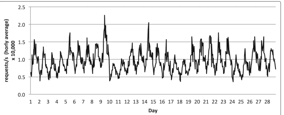
The input data chosen to train the forecasting model and evaluate our proposal were obtained from real web service logs from the Complutense University of Madrid. These data were gathered over a four-week period on an hourly basis. To emulate a server with high data traffic load, the data collected have been extrapolated one order of magnitude. These input training data, summarized in Fig. 3, represent the hourly average load (expressed in requests per second) of the server.
Parameter selection for the SVM forecasting model
The basic parameters of a time-series forecasting model (see “Time series training data” section) are: the size of the training data (N), the lag period (T), and the forecast-ing horizon. The trainforecast-ing data set must be large enough to capture the time series behavior, so in this work we have collected data from a 4-week period, i.e.,N = 672 hours. To choose an appropriate lag period, we analyzed the seasonal patterns of the time series, by measuring the autocorrelation of the input training data, shown in Fig.4. As we can see, the input data exhibit a clear autocorrela-tion for a lag interval of 24 h. For this reason, the chosen lag period wasT =24 hours. Finally, the forecasting hori-zon chosen in our model was one hour, i.e., based on the last N observations, the forecasting model predicts the value of the time series for the next hourly period. We chose this horizon because, in general, the accuracy of the prediction worsens as the forecasting horizon increases, so it is more accurate to apply the forecasting model and make a new prediction each hour. Furthermore, in this work, we obtained these hourly predictions for a test inter-val of 24 h. For this test interinter-val, the real inter-values of the time series were known, so we were able to compare the pre-dicted values with the real values, allowing us to validate the forecasting model.
Besides these basic parameters, the SVM
regres-sion model presented in The support vector regression
modelsection uses some additional configuration param-eters that must be adjusted by the user. In particular,
the C parameter of the regularized risk in Eq. 2, the
Fig. 3Summary of input training data. This graph displays the input data used for the training of the SVM-based forecasting model presented in this work. This data were obtained from real web service logs from the Complutense University of Madrid and were gathered over a four-week period on an hourly basis. To emulate a server with high data traffic load, the data collected have been extrapolated one order of magnitude. These input training data represent the hourly average load (expressed in requests per second) of the server for a 4-week period (i.e.,N=672 hours)
The value of the regularization parameter, C, can be related to the range of response values in the training data. Therefore, according to [47], it can be chosen as follows:
C=max |¯y+3σy|,|¯y−3σy| (16)
where¯yandσyare the mean and standard deviation of the yvalues of training data.
On the other hand, the parameter should be
propor-tional to the input noise level and should also depend on
the number of training samples. According to [47], it can be chosen as follows:
=3σ
lnn
n (17)
where nis the number of samples in the training input
data, and σ is the estimated noise variance observed
from the training data, which can be obtained by fitting the input data using a low-bias model, such as a linear
estimator. In our case, we used a first order linear regres-sion model to estimate theyvalues of the training data, so the estimated noise variance can be computed as follows:
σ2= 1
n−1 n
i=1 yi− ˆyi
2
(18)
Finally, theγ parameter of RBF kernel function should be selected to reflect the range of the input training data, and can be chosen as follows:
γ ∼[0.1−0.5]×range(x) (19)
whererange(x)=max(x)−min(x)for the input training data.
Using the input data shown in Fig. 3, and applying
the previous formulation for the SVM regression model parameters, we obtained the values displayed in Table1.
Forecasting results
The prediction models presented in this work forecast the average hourly load of a distributed server for a 24 h test interval, based on the historical data shown in Fig.3, using the parameters specified in the previous section.
The experimental environment used in this work to run the SVM regression models is based on the WEKA tool [54] from Waikato University, with the time series analysis package.
The results of this section are intended to prove that the SVM regression model outperforms other simpler forecasting methods. For this reason, we compared the behavior of the SVM-based models with the following three simple forecasting methods:
• Forecasting model #1 (based on the last value). The estimated value of the server load in the current time interval is equal to the value in the previous time interval, i.e.,yˆ(t)=y(t−1).
• Forecasting model #2 (based on a simple moving average). The estimated value of the server load in the current time interval was computed as the moving average (MA ) of order three (i.e., anMA(p)
model, withp=3).
• Forecasting model #3 (based on linear regression). The estimated value of the server load in the current time interval was computed using an autoregressive
Table 1Selected values for the SVM parameters
Parameter Value
C 1.9
0.027
γ [ 0.2−1.0]
(AR ) model with a lag period of 24 h (i.e., anAR(p)
model, withp=24)
In addition to these basic methods, we also evaluated the SVM-based forecasting models using three different kernel functions:
• Forecasting model #4 (SVM with a polynomial kernel). This is based on SVM regression with a polynomial kernel (see Eq.6) of orderp=1. We empirically tested higher order polynomials kernels, but they offered no better results than orderp=1, and took more time to execute.
• Forecasting model #5 (SVM with a normalized polynomial kernel). This is based on SVM regression with a normalized polynomial kernel (see Eq.7) of orderp=2. As in the previous case, polynomials kernels of higher orders did not outperform order
p=2, and took more time to execute.
• Forecasting models #6 to #8 (SVM with a RBF kernel). This is based on SVM regression with a RBF kernel (see Eq.8). According to Table1, the optimal values for theγ parameter are between 0.2 and 1.0, so we executed the forecasting algorithm using three different values of this parameter: low value (γ =0.2), medium value (γ =0.6), high value (γ =1.0), corresponding to forecasting models #6, #7, and #8, respectively.
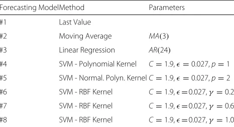
A summary of all the forecasting methods used in this work is shown in Table2.
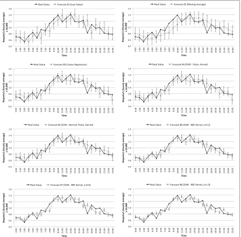
Figure5shows the prediction results for the 24 h test interval using the various forecasting methods compared to the real values of the average server load for the same hours. The error bars of the different graphs represent the expected error of the model computed as the RMSE of the training data for each time interval.
Figure6shows the accuracy of the different forecasting models for the 24 h test interval, where the MAE, MSE, and RMSE values represent the real prediction error of each forecasting model for this period.
Table 2Summary of different forecasting models
Forecasting ModelMethod Parameters
#1 Last Value
#2 Moving Average MA(3)
#3 Linear Regression AR(24)
#4 SVM - Polynomial Kernel C=1.9,=0.027,p=1
#5 SVM - Normal. Polyn. KernelC=1.9,=0.027,p=2
#6 SVM - RBF Kernel C=1.9,=0.027,γ=0.2
#7 SVM - RBF Kernel C=1.9,=0.027,γ=0.6
Fig. 5Predicted server loads obtained with different forecasting models (#1 to #8). This figure shows the prediction results for the 24 h test interval using the various forecasting models (#1 to #8) compared to the real values of the average server load for the same hours. The bar errors of the different graphs represent the expected error (RMSE) of the model. This is computed as the error between the estimated data obtained by the forecasting model for the training period and the real training data of the time series
As we can see, SVM-based forecasting (models #4 to #8) is more accurate than the three basic methods (mod-els #1 to #3), as prediction errors (MAE, MSE, and RMSE) are lower in all cases. In addition, if we compare the
SVM-based methods, the RBF kernel withγ = 0.2 and
γ =1.0 (models #6 and #8) obtains better results than the polynomial kernels.
Resource allocation results
Once the server load predictions had been obtained, based on the different forecasting models, we were able to apply the M/M/c queue performance model
presented in Performance model section to obtain
Fig. 6Accuracy of different forecasting models (real prediction error for the forecasting period) This figure shows the accuracy of the different forecasting models for the 24 h test interval (forecasting horizon), where the MAE, MSE, and RMSE values represent the real prediction error of each forecasting model for this period. They are computed as the error between the data obtained by the forecasting model and the real data of the time series for the forecasting horizon
the expected load and fulfill the SLA contracted by the user, expressed in terms of maximum response time.
In addition, as we know the real hourly load of the server for the 24 h test interval, we were able to compare the optimal number of resources that should be provi-sioned based on the real load, calledoptimal allocation, with the estimated resource allocation based on the fore-casted loads, calledestimated allocation. We were there-fore able to determine, for each there-forecasting model and each hourly period, whether the server was being over-provisioned (whereestimated allocation>optimal allo-cation), under-provisioned (where estimated allocation < optimal allocation)), or correctly provisioned (where estimated allocation=optimal allocation).
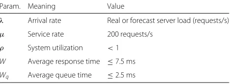
To apply the M/M/c model, we first defined the param-eters to be used in the model, summarized in Table3:
• The arrival rate (λ) is the average load of the server (expressed in requests/s) each hour. We considered the predicted load obtained for each one of the
Table 3M/M/c queueing model parameters
Param. Meaning Value
λ Arrival rate Real or forecast server load (requests/s)
μ Service rate 200 requests/s
ρ System utilization <1 W Average response time ≤7.5 ms
Wq Average queue time ≤2.5 ms
forecasting models for the 24 h test interval, as well as the real load of the server for the same period.
• The service rate (μ) is the number of requests that each backend server can process per time unit. In this work, we assumed a value ofμ=200requests/s for each backend server. This is a typical throughput value of a mid-range server (e.g., an Amazon EC2 medium instance) serving dynamic content requests (e.g., PHP) [55,56].
• The system utilization factor (ρ) must be less than 1 to guarantee system stability. The number of
provisioned resources must be sufficient to guarantee this condition.
• The average queue time (Wq) and the average response time (W=1/μ+Wq), which are limited
by the SLA contracted by the user. In this work, we assumed that the user SLA established a limit value forWq that could not exceed 50% of the minimum response time, i.e.,Wq≤0.5×1/μ=2.5ms. Hence,
the maximum response time (W ) imposed by the SLA was 7.5 ms.
Next, using the real and forecast server load values obtained by the different forecasting models as input (i.e. real and forecastλvalues), we applied the M/M/c queu-ing model to determine the number of resources (backend servers) that must be provisioned, in order to guarantee system stability (ρ <1) and fulfill the maximum response time imposed by the SLA (W≤7.5 ms).
of provisioned resources; ii) the number of SLA vio-lations; and iii) the number of unserved requests. We considered that the SLA of a request is violated when its response time isW > 7.5 ms. In addition, we also estab-lished a maximum limit (time-out) of 1 s for serving a request, so that if the response time exceeds this limit, the request is considered as unserved. Form the point of view of the user, the optimal resource allocation is the one that minimize the number of resources, and hence the cost of the infrastructure, while also minimize the number of SLA violations, and the number of unserved request. When the number of provisioned resources is too low (under-provisioning) the cost of the infrastructure decreases, but the number of SLA violations and unserved requests increases. On the other hand, if the number of provisioned resources is too high (over-provisioning), the number of SLA violations and unserved requests would be negligible, but the cost of the infrastructure shoots up.
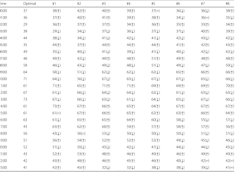
Table4shows the hourly results of the provisioning for
the 24 h test interval. The Optimal column shows the
optimal allocation results based on the real load of the server. Columns "#1" to "#8" show the estimated allo-cation results computed from the predicted server loads (i.e., the central load values displayed in Fig. 5 for the forecasting models #1 to #8, respectively). For these eight columns, this table also relates whether the system is being over-provisioned (↑), under-provisioned (↓), or correctly provisioned (=).
Regarding the number of provisioned resources in
Table 4, we can see that, in most cases, the
esti-mated allocation value based on SVM forecasting models (columns #4 to #8) is closer to the opti-mal value than the simple forecasting models (columns
#1 to #3). This fact is most evident in Fig. 7,
which shows the total number of over-provisioned and under-provisioned resources over the 24 h test interval.
If we look at the total number of over-provisioned resources, we can see that the SVM-based models (#4 to #8) outperform the simple forecasting methods (#1 to #3);
forecasting model #6 (SVM - RBF Kernel, λ = 0.2) is
Table 4Allocation 1: Optimal resource allocation (based on real load) vs. estimated resource allocation (based on predicted loads, forecasting models #1 to #8)
Time Optimal #1 #2 #3 #4 #5 #6 #7 #8
00:00 37 38(↑) 42(↑) 40(↑) 39(↑) 37(=) 36(↓) 36(↓) 38(↑)
01:00 36 37(↑) 40(↑) 41(↑) 39(↑) 38(↑) 34(↓) 36(=) 35(↓)
02:00 29 36(↑) 37(↑) 37(↑) 34(↑) 36(↑) 35(↑) 33(↑) 34(↑)
03:00 38 29(↓) 34(↓) 37(↓) 36(↓) 37(↓) 37(↓) 40(↑) 39(↑)
04:00 44 38(↓) 34(↓) 41(↓) 42(↓) 41(↓) 42(↓) 43(↓) 42(↓)
05:00 35 44(↑) 37(↑) 44(↑) 44(↑) 44(↑) 41(↑) 42(↑) 43(↑)
06:00 49 35(↓) 40(↓) 41(↓) 39(↓) 41(↓) 40(↓) 42(↓) 42(↓)
07:00 46 49(↑) 42(↓) 49(↑) 48(↑) 51(↑) 49(↑) 48(↑) 48(↑)
08:00 58 46(↓) 43(↓) 49(↓) 48(↓) 51(↓) 49(↓) 47(↓) 50(↓)
09:00 64 58(↓) 51(↓) 62(↓) 62(↓) 62(↓) 65(↑) 66(↑) 66(↑)
10:00 71 64(↓) 56(↓) 67(↓) 65(↓) 67(↓) 67(↓) 65(↓) 66(↓)
11:00 61 71(↑) 65(↑) 71(↑) 71(↑) 69(↑) 69(↑) 69(↑) 70(↑)
12:00 67 61(↓) 66(↓) 64(↓) 64(↓) 62(↓) 61(↓) 63(↓) 63(↓)
13:00 73 67(↓) 66(↓) 63(↓) 61(↓) 64(↓) 65(↓) 67(↓) 66(↓)
14:00 61 73(↑) 67(↑) 66(↑) 65(↑) 64(↑) 67(↑) 67(↑) 67(↑)
15:00 61 61(=) 67(↑) 66(↑) 65(↑) 62(↑) 63(↑) 66(↑) 64(↑)
16:00 63 61(↓) 65(↑) 65(↑) 64(↑) 60(↓) 58(↓) 55(↓) 57(↓)
17:00 43 63(↑) 62(↑) 60(↑) 59(↑) 57(↑) 58(↑) 57(↑) 56(↑)
18:00 56 43(↓) 56(=) 53(↓) 50(↓) 50(↓) 50(↓) 51(↓) 51(↓)
19:00 51 56(↑) 54(↑) 52(↑) 52(↑) 52(↑) 49(↓) 45(↓) 46(↓)
20:00 52 51(↓) 50(↓) 43(↓) 42(↓) 47(↓) 44(↓) 44(↓) 45(↓)
21:00 43 52(↑) 53(↑) 48(↑) 46(↑) 49(↑) 46(↑) 49(↑) 49(↑)
22:00 42 43(↑) 48(↑) 46(↑) 45(↑) 46(↑) 40(↓) 42(=) 42(=)
Fig. 7Over- and under-provisioning of resources using different forecasting models, based on the resource allocation of Table4This figure shows the total number of over-provisioned and under-provisioned resources over the 24 h test interval for the different forecasting models (#1 to #8), based on the resource allocation of Table4. This is computed as the difference between the number of resources that should be provisioned according to the predicted load of the different forecasting models, and the optimal number of resources that should be provisioned according to the real load of the server for the 24 h test interval
the best case. If we look at the total number of under-provisioned resources, the best forecasting methods are, once again, the SVM-based forecasting models #5 (SVM - Normal. Polynomial Kernel) and #8 (SVM - RBF Kernel, λ=1.0).
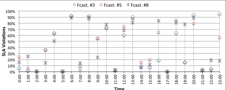
Figures 8 and 9 show, respectively, the percentage of SLA violations and unserved requests on each hourly period for forecasting models #3, #5, and #8 (in order to avoid a mesh of points in the graph, we have chosen these three cases in representation of the basic models, the polynomial SVM-based models, and the RBF SVM-based models, respectively). In addition, Table5shows the total
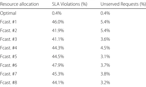
number of SLA violations and unserved requests over the 24 h test interval, expressed as a percentage with respect the total number of requests.
Regarding the SLA violations results, we can see that all the forecasting models produce a high number of SLA violations: between 40% and 50% of the total number of requests, as shown in Table5. This is because all the fore-casting models cause under-provisioning of resources in several hourly periods (about half of the periods in most cases). This under-provisioning results in a high num-ber of SLA violations, which can reach, in some cases, almost the 100% of requests, as shown in Fig. 8. If we
Fig. 9Percentage of unserved requests for forecasting models #3, #5, and #8, based on the resource allocation of Table4This figure shows the percentage of unserved requests on each hourly period for forecasting models #3, #5, and #8 (in order to avoid a mesh of points in the graph, we have chosen these three cases in representation of the basic models, the polynomial SVM-based models, and the RBF SVM-based models, respectively)
compare the percentage of total SLA violations of the dif-ferent forecasting models in Table5, we can see that two of the basic forecasting models (specifically, models #2 and #3) behave slightly better than the SVM-based models. This is because the number of hourly periods with a high shortage of resources for these two forecasting models is lower than for other models.
On the other hand, regarding the unserved requests results in Fig.9, we can see that in most hourly periods the percentage of unserved requests is negligible, and only in a few periods this percentage exceeds 10%. Regarding the percentage of total unserved requests in Table5, we can see that most SVM-based models outperforms the basic models, being forecasting models #5 and #8 those that present the best behavior.
Table 5Percentage of SLA violations and unserved requests over total number of requests for the 24 h test interval, based on the resource allocation of Table4
Resource allocation SLA Violations (%) Unserved Requests (%)
Optimal 0.4% 0.4%
Fcast. #1 46.0% 5.4%
Fcast. #2 41.9% 5.4%
Fcast. #3 41.1% 3.6%
Fcast. #4 44.3% 4.5%
Fcast. #5 44.5% 3.1%
Fcast. #6 47.9% 3.7%
Fcast. #7 45.3% 3.8%
Fcast. #8 44.1% 3.2%
We can conclude that the models that perform better are those that minimize the number of under-provisioning periods and under-provisioned resources (so reducing the number of SLA violations, and unserved requests), but at the same time they do not exceed too much the number of over-provisioned resources (so avoiding a significant infrastructure cost increasing). Therefore, the SVM-based forecasting models #5 and #8 exhibit the best trade-off for the three considered metrics (number of resources, num-ber of SLA violations, and numnum-ber of unserved requests). However, it is important to notice that them basic model #3 also present a good trade-off of the three metrics and a better behavior regarding SLA violations.
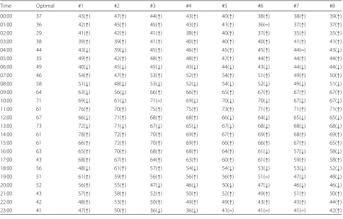
In order to reduce the number of SLA violations, we achieved a second resource allocation based on the pre-dicted load values displayed on Fig.5, but instead of using the central load values of the graphs, we used the central load values plus half the expected error (represented by the error bars in Fig.5). Table6shows the hourly results of this new provisioning, and Fig.10shows the total num-ber of over-provisioned and under-provisioned resources over the 24 h test interval.
Regarding the number of over-provisioned resources, we can see that SVM-based forecasting models outper-forms the basic models, being forecasting models based on RBF Kernel (models #6, #7, and #8) the ones that behave better. However, these models do not offer the best results regarding the number of under-provisioned resources, in fact, models #7 and #8 are the worst cases, while forecasting models #3 and #5 are the ones with less number of under-provisioned resources.
Table 6Allocation 2: Optimal resource allocation (based on real load) vs. estimated resource allocation (based on predicted loads plus half the expected error, forecasting models #1 to #8)
Time Optimal #1 #2 #3 #4 #5 #6 #7 #8
00:00 37 43(↑) 47(↑) 44(↑) 43(↑) 40(↑) 38(↑) 38(↑) 39(↑)
01:00 36 42(↑) 45(↑) 45(↑) 43(↑) 41(↑) 36(=) 37(↑) 37(↑)
02:00 29 41(↑) 42(↑) 41(↑) 38(↑) 40(↑) 37(↑) 35(↑) 35(↑)
03:00 38 39(↑) 39(↑) 41(↑) 40(↑) 40(↑) 40(↑) 41(↑) 41(↑)
04:00 44 43(↓) 39(↓) 45(↑) 46(↑) 45(↑) 45(↑) 44(=) 43(↓)
05:00 35 49(↑) 42(↑) 48(↑) 48(↑) 47(↑) 44(↑) 44(↑) 44(↑)
06:00 49 40(↓) 45(↓) 45(↓) 43(↓) 44(↓) 43(↓) 44(↓) 44(↓)
07:00 46 54(↑) 47(↑) 53(↑) 52(↑) 54(↑) 51(↑) 49(↑) 50(↑)
08:00 58 51(↓) 48(↓) 53(↓) 52(↓) 54(↓) 52(↓) 49(↓) 51(↓)
09:00 64 63(↓) 56(↓) 66(↑) 66(↑) 65(↑) 67(↑) 67(↑) 67(↑)
10:00 71 69(↓) 61(↓) 71(=) 69(↓) 70(↓) 70(↓) 67(↓) 67(↓)
11:00 61 76(↑) 70(↑) 75(↑) 75(↑) 73(↑) 71(↑) 71(↑) 71(↑)
12:00 67 66(↓) 71(↑) 68(↑) 68(↑) 66(↓) 64(↓) 65(↓) 65(↓)
13:00 73 72(↓) 71(↓) 67(↓) 65(↓) 67(↓) 68(↓) 68(↓) 68(↓)
14:00 61 78(↑) 72(↑) 70(↑) 69(↑) 67(↑) 69(↑) 68(↑) 69(↑)
15:00 61 66(↑) 72(↑) 70(↑) 69(↑) 66(↑) 66(↑) 67(↑) 65(↑)
16:00 63 65(↑) 70(↑) 68(↑) 68(↑) 64(↑) 61(↓) 57(↓) 58(↓)
17:00 43 68(↑) 67(↑) 64(↑) 63(↑) 60(↑) 61(↑) 59(↑) 58(↑)
18:00 56 48(↓) 61(↑) 57(↑) 54(↓) 54(↓) 53(↓) 53(↓) 52(↓)
19:00 51 61(↑) 59(↑) 56(↑) 56(↑) 56(↑) 51(=) 47(↓) 48(↓)
20:00 52 56(↑) 55(↑) 47(↓) 46(↓) 50(↓) 47(↓) 46(↓) 46(↓)
21:00 43 57(↑) 58(↑) 52(↑) 50(↑) 52(↑) 49(↑) 51(↑) 50(↑)
22:00 42 48(↑) 53(↑) 50(↑) 49(↑) 49(↑) 43(↑) 43(↑) 44(↑)
23:00 41 47(↑) 50(↑) 36(↓) 36(↓) 41(=) 41(=) 41(=) 42(↑)
shown in Table 7, we can see that the percentage of total SLA violations in all the cases is considerably lower than in the first resource allocation: between 8% for the best case (forecasting model #3) and about 34% for the two worst cases (forecasting models #7 and #8). Similarly, unserved requests have been also significantly reduced with regard to the first resource allocation, being forecasting models #3 and #5 the two best cases, with a negligible number of unserved requests.
In conclusion, we can assert that, in general, SVM-based forecasting models outperform basic forecast-ing models regardforecast-ing the number of over-provisioned resources. However, regarding the number of SLA vio-lations and unserved requests, some of the SVM-based models have worse results than basic models. Accord-ing to the results of the second allocation, based on the predicted load values plus half the expected error, the model that offers the best tradeoff of the three con-sidered metrics (number of resources, number of SLA violations, and number of unserved requests) is the forecasting model #5 (SVM - normalized polynomial model).
Finally, it is important to remark that the execution of the proposed auto-scaling mechanism, including both the server load forecast (using basic or SVM-based models), and the resource estimation, takes only a few seconds (less than one minute in the worst case). Furthermore, using the appropriate techniques, cloud resource instances can also be provisioned or de-provisioned in a matter of sec-onds [57–59]. Therefore, auto-scaling actions (including startup/shutdown of resource instances) can be done with a minimum delay, typically between 1 and 5 min. To deal with this delay, and taking into account that we use an auto-scaling period of an hour, we can call the auto-scaler a few minutes before the next auto-scaling period, so that the required resources are ready when this period begins.
Table 7Percentage of SLA violations and unserved requests over total number of requests for the 24 h test interval, based on the resource allocation of Table6
Resource allocation SLA Violations (%) Unserved Requests (%)
Optimal 0.4% 0.4%
Fcast. #1 11.2% 0.4%
Fcast. #2 15.2% 0.7%
Fcast. #3 10.8% 0.1%
Fcast. #4 17.6% 0.5%
Fcast. #5 8.0% 0.1%
Fcast. #6 19.3% 0.5%
Fcast. #7 34.6% 1.5%
Fcast. #8 33.6% 1.3%
Conclusion and future work
In this paper, we have presented an auto-scaling method for adaptive provisioning of elastic cloud services, based on ML time-series forecasting and queuing theory, aimed at optimizing the latency (response time) of the service, and reducing over-provisioning. The auto-scaling system uses a SVM regression to predict the processing load of a web server, based on historical observations. Before apply-ing the SVM regression model, we fine-tuned its param-eters, allowing us to capture the nonlinear and temporal patterns of the input data, and achieve an accurate predic-tion. Using the historical load values of a real web service as input data, we applied the SVM forecasting model using various kernel functions (polynomial kernel, normalized polynomial kernel, and RBF kernel) and different config-uration parameters. We compared the accuracy of these predictions with those obtained from other simple meth-ods (last value, MA, and AR models), by computing the MAE and RMSE error measurements for the 24 h test interval. Our results show that the SVM-based regres-sion model has better prediction accuracy than the simple methods.
In addition, the proposed auto-scaling mechanism com-bines the SVM forecasting method with a M/M/c queue-based performance model. This allowed us to estimate the appropriate number of resources that must be provi-sioned, according to the predicted load, in order to reduce the service time, and fulfill the SLA contracted by the user. The experimental results also show that, in general, resource allocations based on SVM forecasting are closer to the optimal allocation (based on real load observa-tions) than those based on simple forecasting methods. In particular, SVM forecasting models based on normalized polynomial kernels give the best allocation results with regard to the number of over-provisioned resources, the number of SLA violations, and the number of unserved requests.
As future work, we plan to extend both the fore-casting and performance models to other distributed services, such as big data clusters (e.g., Hadoop or Spark clusters), with the goal of implementing effi-cient auto-scaling mechanisms for these architectures. The forecasting and performance models should be adapted to the particularities and functionality of the different components in these kinds of clus-ters, such as Mapreduce, HDFS, YARN, and Spark components.
Abbreviations
Agreement; SLO: Service Level Objective; SVM: Support Vector Machine; YARN: Yet Another Resource Negotiator
Acknowledgements
Not applicable.
Funding
This research was supported by the Comunidad de Madrid (Spain), through research grant P2018/TCS4499. This funding allowed us to acquire the computing resources needed for completing this research.
Availability of data and materials
The input data chosen to train and evaluate the forecasting model proposed in this work were obtained from real web service logs from the Complutense University of Madrid. These input and test data sets are available as supplementary material to this manuscript and also athttps://goo.gl/Jez9Kg.
Authors’ contributions
RMV conceived the study, carried out its design, conducted the experimental section, and drafted the manuscript. RSM participated in the definition and implementation of the experimental section, and helped to refine the manuscript. EH participated in the definition and implementation of the queue-based performance model, and also helped to refine the manuscript. IML coordinated the research, participated in the analysis of different SVM-based methods, and helped to draft and refine the manuscript. All authors read and approved the final manuscript.
Authors information
Not applicable.
Competing interests
The authors declare that they have no competing interests.
Publisher’s Note
Springer Nature remains neutral with regard to jurisdictional claims in published maps and institutional affiliations.
Author details
1Computer Science School, Complutense University, 28040 Madrid, Spain. 2IACS/SEAS, Harvard University, 02138 MA Cambridge, USA.
Received: 9 December 2018 Accepted: 29 March 2019
References
1. Herbst N, Kounev S, Reussner R (2013) Elasticity in cloud computing: What it is, and what it is not. In: Proceedings of the 10th International Conference on Autonomic Computing (ICAC 13). USENIX, San Jose. pp 23–27
2. Beloglazov A, Abawajy J, Buyya R (2012) Energy-aware resource allocation heuristics for efficient management of data centers for cloud computing. Futur Gener Comput Syst 28(5):755–768. Special Section: Energy efficiency in large-scale distributed systems
3. Dougherty B, White J, Schmidt D (2012) Model-driven auto-scaling of green cloud computing infrastructure. Futur Gener Comput Syst 28(2):371–378
4. Ye K, Huang D, Jiang X, Chen H, Wu S (2010) Virtual machine based energy-efficient data center architecture for cloud computing: A performance perspective. In: Green Computing and Communications (GreenCom) 2010 IEEE/ACM Int’l Conference on Int’l Conference on Cyber, Physical and Social Computing (CPSCom). pp 171–178
5. Papadopoulos A, Ali-Eldin A, Årzén K, Tordsson J, Elmroth E (2016) Peas: A performance evaluation framework for auto-scaling strategies in cloud applications. ACM Trans Model Perform Eval Comput Syst 1(4):15:1–15:31 6. Lorido-Botran T, Miguel-Alonso J, Lozano JA (2014) A review of
auto-scaling techniques for elastic applications in cloud environments. J Grid Comput 12(4):559–592
7. Jiang J, Lu J, Zhang G, Long G (2013) Optimal cloud resource auto-scaling for web applications. In: 2013 13th IEEE/ACM International Symposium on Cluster, Cloud, and Grid Computing. ACM, New York. pp 58–65 8. Messias V, Estrella JC, Ehlers R, Santana MJ, Santana RC, Reiff-Marganiec S
(2016) Combining time series prediction models using genetic algorithm
to autoscaling web applications hosted in the cloud infrastructure. Neural Computing and Applications 27(8):2383–2406
9. Roy N, Dubey A, Gokhale A (2011) Efficient autoscaling in the cloud using predictive models for workload forecasting. In: Proceedings of the 2011 IEEE 4th International Conference on Cloud Computing, CLOUD ’11. IEEE Computer Society, Washington, DC. pp 500–507
10. Verma M, Gangadharan G, Narendra N, Vadlamani R, Inamdar V, Ramachandran L, Calheiros R, Buyya R (2016) Dynamic resource demand prediction and allocation in multi-tenant service clouds. Concurrency and Computation: Practice and Experience 28(17):4429–4442. CPE-15-0088.R1 11. Box G, Jenkins G (1990) Time Series Analysis, Forecasting and Control.
Holden-Day, Incorporated, San Francisco
12. Islam S, Keung J, Lee K, Liu A (2012) Empirical prediction models for adaptive resource provisioning in the cloud. Future Generation Computer Systems 28(1):155–162
13. Jiang Y, Perng C, Li T, Chang R (2012) Self-adaptive cloud capacity planning. In: 2012 IEEE Ninth International Conference on Services Computing. pp 73–80
14. Shevade S, Keerthi S, Bhattacharyya C, Murthy K (2000) Improvements to the smo algorithm for svm regression. IEEE Transactions on Neural Networks 11(5):1188–1193
15. Schölkopf B, Smola A (2002) Learning with Kernels. MIT Press, Cambridge 16. Gross D, Shortle J, Thompson JM, Harris C (2008) Fundamentals of
queueing theory. Wiley, Hoboken
17. Moreno-Vozmediano R, Montero R, Llorente I (2011) Elastic management of web server clusters on distributed virtual infrastructures. Concurrency and Computation: Practice and Experience 23(13):1474–1490
18. Qu C, Calheiros R, Buyya R (2016) A reliable and cost-efficient auto-scaling system for web applications using heterogeneous spot instances. Journal of Network and Computer Applications 65:167–180
19. Cocaña-Fernández A, Sánchez L, Ranilla J (2016) Leveraging a predictive model of the workload for intelligent slot allocation schemes in energy-efficient {HPC} clusters. Engineering Applications of Artificial Intelligence 48:95–105
20. Marosi A, Kovács J, Kacsuk P (2013) Towards a volunteer cloud system. Future Generation Computer Systems 29(6):1442–1451
21. Montero R, Moreno-Vozmediano R, Llorente I (2011) An elasticity model for high throughput computing clusters. Journal of Parallel and Distributed Computing 71(6):750–757
22. Rodero-Merino L, Vaquero LM, Gil V, Galán F, Fontán J, Montero RS, Llorente IM (2010) From infrastructure delivery to service management in clouds. Future Generation Computer Systems 26(8):1226–1240 23. San-Aniceto I, Moreno-Vozmediano R, Montero R, Llorente I (2011) Cloud
capacity reservation for optimal service deployment. In: Proceedings of the The Second International Conference on Cloud Computing, GRIDs, and Virtualization, Rome. IARIA Conference. pp 52–59
24. Gandhi A, Thota S, Dube P, Kochut A, Zhang L (2016) Autoscaling for hadoop clusters. In: 2016 IEEE International Conference on Cloud Engineering (IC2E). MDPI, Basel. pp 109–118
25. Li Z, Yang C, Liu K, Hu F, Jin B (2016) Automatic scaling hadoop in the cloud for efficient process of big geospatial data. ISPRS International Journal of Geo-Information 5(10):173
26. Smowton C, Balla A, Antoniades D, Miller C, Pallis G, Dikaiakos MD, Xing W (2017) A cost-effective approach to improving performance of big genomic data analyses in clouds. Future Generation Computer Systems 67:368–381
27. Moreno-Vozmediano R, Montero R, Llorente I (2012) Iaas cloud architecture: From virtualized data centers to federated cloud infrastructures. Computer 45(12):65–72
28. Hasan M, Magana E, Clemm A, Tucker L, Gudreddi S (2012) Integrated and autonomic cloud resource scaling. In: 2012 IEEE Network Operations and Management Symposium. pp 1327–1334
29. Chieu T, Mohindra A, Karve A (2011) Scalability and performance of web applications in a compute cloud. In: Proceedings of the 2011 IEEE 8th International Conference on e-Business Engineering, ICEBE ’11. IEEE Computer Society, Washington, DC. pp 317–323
30. Lim H, Babu S, Chase J, Parekh S (2009) Automated control in cloud computing: Challenges and opportunities. In: Proceedings of the 1st Workshop on Automated Control for Datacenters and Clouds, ACDC ’09. ACM, New York. pp 13–18
Proceedings of the 4th ACM European Conference on Computer Systems, EuroSys ’09. ACM, New York. pp 13–26
32. Dutreilh X, Kirgizov S, Melekhova O, Malenfant J, Rivierre N, Truck I (2011) Using Reinforcement Learning for Autonomic Resource Allocation in Clouds: towards a fully automated workflow. In: 7th International Conference on Autonomic and Autonomous Systems (ICAS’2011). IARIA, Venice. pp 67–74
33. Tesauro G, Jong NK, Das R, Bennani MN (2006) A Hybrid Reinforcement Learning Approach to Autonomic Resource Allocation. In: Proceedings of the 2006 IEEE International Conference on Autonomic Computing (ICAC). IEEE Computer Society, Washington, DC. pp 65–73
34. Barrett E, Howley E, Duggan J (2013) Applying reinforcement learning towards automating resource allocation and application scalability in the cloud. Concurrency and Computation: Practice and Experience 25(12):1656–1674
35. Salah K, Elbadawi K, Boutaba R (2016) An analytical model for estimating cloud resources of elastic services. Journal of Network and Systems Management 24(2):285–308
36. Kaur PD, Chana I (2014) A resource elasticity framework for qos-aware execution of cloud applications. Future Generation Computer Systems 37:14–25. Special Section: Innovative Methods and Algorithms for Advanced Data-Intensive ComputingSpecial Section: Semantics, Intelligent processing and services for big dataSpecial Section: Advances in Data-Intensive Modelling and SimulationSpecial Section: Hybrid Intelligence for Growing Internet and its Applications
37. Ahmed N, Atiya A, Gayar NE, El-Shishiny H (2010) An empirical comparison of machine learning models for time series forecasting. Econometric Reviews 29(5-6):594–621
38. Bontempi G, Taieb S, Borgne YL (2013) Business Intelligence: Second European Summer School, eBISS 2012, Brussels, Belgium, July 15-21, 2012,. Springer Berlin Heidelberg, Berlin
39. Allende H, Moraga C, Salas R (2002) Artificial neural networks in time series forecasting: a comparative analysis. Kybernetika 38(6):685–707 40. Zhang G (2003) Time series forecasting using a hybrid {ARIMA} and neural
network model. Neurocomputing 50:159–175
41. Thissen U, van Brakel R, de Weijer A, Melssen W, Buydens L (2003) Using support vector machines for time series prediction. Chemometrics and Intelligent Laboratory Systems 69(1–2):35–49
42. Müller K, Smola A, Rätsch G, Schölkopf B, Kohlmorgen J, Vapnik V (1997) Artificial Neural Networks – ICANN’97: 7th International Conference Lausanne, Switzerland, October 8–10, 1997. In: Proceedings chap. Predicting time series with support vector machines. Springer Berlin Heidelberg. pp 999–1004
43. Burges C (1998) A tutorial on support vector machines for pattern recognition. Data Mining and Knowledge Discovery 2(2):121–167 44. Smola A, Schölkopf B (2004) A tutorial on support vector regression.
Statistics and Computing 14:199–222
45. Suykens J, Vandewalle J (1999) Least squares support vector machine classifiers. Neural Processing Letters 9(3):293–300
46. Vapnik V (1998) Statistical Learning Theory. Wiley-Interscience, New York 47. Cherkassky V, Ma Y (2004) Practical selection of svm parameters and noise
estimation for svm regression. Neural Netw. 17(1):113–126
48. Shawe-Taylor J, Cristianini N (2004) Kernel Methods for Pattern Analysis. Cambridge University Press, New York
49. Üstün B, Melssen W, Buydens L (2006) Facilitating the application of support vector regression by using a universal pearson {VII} function based kernel. Chemometrics and Intelligent Laboratory Systems 81(1):29–40 50. Rauber T, Berns K (2011) Kernel multilayer perceptron. IEEE Computer
Society, Washington
51. Boardman M, Trappenberg T (2006) A heuristic for free parameter optimization with support vector machines. In: The 2006 IEEE International Joint Conference on Neural Network Proceedings. pp 610–617 52. Cassabaum M, Waagen D, Rodriguez J, Schmitt H (2004) Unsupervised
optimization of support vector machine parameters. In: Proceedings of SPIE 5426, Automatic Target Recognition XIV. SPIE, Bellingham. pp 316–325
53. Chapelle O, Vapnik V, Bousquet O, Mukherjee S (2002) Choosing multiple parameters for support vector machines. Machine Learning 46(1):131–159 54. Frank E, Hall M, Holmes G, Kirkby R, Pfahringer B (2005) WEKA–A machine
learning workbench for data mining. Springer, Boston
55. Iqbal W, Dailey M, Carrera D, Janecek P (2011) Adaptive resource provisioning for read intensive multi-tier applications in the cloud. Future Gener. Comput. Syst. 27(6):871–879
56. Kujawa L (2013) Performance benchmark of popular php frameworks. https://systemsarchitectdotnet.wordpress.com/2013/04/23/performance-benchmark-of-popular-php-frameworks/. Posted on April 23
57. Razavi K, Kolk GVD, Kielmann T (2015) PrebakedμVMs: scalable, instant VM startup for IaaS clouds. In: Proceedings of the 35th IEEE International Conference on Distributed Computing Systems. pp 245–255 58. Razavi K, Costache S, Gardiman A, Verstoep K, Kielmann T (2015) Scaling
VM deployment in an open source cloud stack. In: Proceedings of the 6th Workshop on Scientific Cloud Computing