Model-based learning of information diffusion in social media networks

R E S E A R C H

Open Access

Model-based learning of information

diffusion in social media networks

Zhecheng Qiang

, Eduardo L. Pasiliao

and Qipeng P. Zheng

*Correspondence: [email protected] 1_{Department of Industrial} Engineering and Management Systems, University of Central Florida, Orlando 32826, FL, USA Full list of author information is available at the end of the article

Abstract

Social media networks have become widely used platforms for their users to share information. Learning the information diffusion process is essential for successful applications of viral marketing and cyber security in social media networks. This paper proposes two learning models that are aimed at learning person-to-person influence in information diffusion from historical cascades based on the threshold propagation model. The first model is based on the linear threshold propagation model. In addition, by considering multi-step information propagation in one time period, this paper proposes a learning model for multi-step diffusion influence between pairs of users based on the idea of random walk. Mixed integer programs (MIP) have been used to learn these models by minimizing the prediction errors, where decision variables are estimations of the diffusion influence between pairs of users. For large-scale networks, this paper develops approximate methods for those learning models by using artificial neural networks to learn the pairwise influence. Extensive computational experiments using both synthetic data and real data have been conducted to demonstrate the effectiveness of the proposed models and methods.

Keywords: Social media networks, Information diffusion, Machine learning, Mixed integer programming, Artificial neural network, Optimization

Introduction

The rapid development of the Internet and its mobile computing technologies in the past several decades contributes to form online virtual communities in social media net-works. People share news, their ideas, interests and information in social media netnet-works. Understanding how the information propagates is essential for successful applications of viral marketing (Domingos2005) and cyber security (Budak et al.2011) in social media networks. To this end, researchers have defined different problems such as the influ-ence maximization problem (Kempe et al.2003; Kimura et al.2007) and contamination minimization problem (Kimura et al. 2009). Influence maximization problem involves finding a limited number of nodes which have the largest influence. Similarly, contamina-tion minimizacontamina-tion problem involves blocking a limited number of nodes which suppress the propagation of the rumors. However, all of the parameters in the diffusion models are assumed to be known. In reality, these parameters are not readily available from the massive historical datasets of social media networks. To fill this gap, this paper proposes several models to learn these influence parameters from historical cascades.

In the literature, researchers have tried to learn the information diffusion processes through different diffusion models. There are two most prevalent diffusion models - Inde-pendent Cascade Model (IC) (Kempe et al.2003) and General Threshold Model (GT) (Granovetter1978). In the Independent Cascade Model, each active parent nodeihas a single chance to activate the child nodejwith a diffusion probabilitypi,j. Satio et al.

(2008) studied the problem of learning influence probabilities based on the IC propa-gation model. They estimated the diffusion probabilities by expectation-maximization algorithm where the likelihood was maximized by iteratively updating the parameters. Besides, there are some variants of Independent Cascade model based research, consid-ering continuous time delays of infection as well (Saito et al.2009; Rodriguez et al.2011). In contrast to IC models, General Threshold Model assumes that an inactive userjin social media networks is activated by all of its active neighbors when the total influence is larger than the target user’s threshold. Linear Threshold Model is a special case of General Threshold Model and the total influence is the sum of the influence weights of activated neighbors. Goyal et al. (2010) adopted the General Threshold diffusion Model and pro-posed three probabilistic models, which were Bernoulli distribution, Jaccard Index and Partical Credits to predict the diffusion influence weights. (Vaswani S, Duttachoudhury N: Learning influence diffusion probabilities under the linear threshold model, unpublished) learned the influence diffusion weights under the Linear Threshold Model. They used three different methods, i.e, gradient descent, interior point method and EM algorithm to maximize the likelihood estimate.

In this paper, we propose two different mixed-integer programming models to esti-mate the diffusion influence weights between pairs of users underlying the threshold model. We learn the diffusion influence weights through mining past diffusion cas-cades of posts. Given the historical information cascading data containing the initial statesx0_i and final statesxT_i of all the nodes which are users in social media networks, we are trying to learn the diffusion influence weights wi,j between pairs of users in

the Threshold Models. Two different learning models are built under the assumption. The first model is based on the Linear Threshold Model, where a user will be acti-vated when the sum of its neighbors’ influence weight is larger than the threshold of the user. The second model considers multi-step influence from the multi-hop neigh-borhood of the user. In the real dataset, the status of nodes at each time step could be collected. However, the time required for each propagation varies. When we know the status of users at two different time steps, the propagation steps could be more than one. Therefore, it’s necessary to consider multi-step influence to better fit the real data.

We summarize the contributions of this paper as follows,

• We propose two mixed-integer programming models to learn diffusion influence between pairs of users. One is based on the popular propagation model, i.e., Linear Threshold Model, and another one is based on the idea of random walk considering multi-step influence.

• For large-scale network, we come up with approximate methods for the two learning models using artificial neural networks with no hidden layer.

The remainder of the article is organized as follows. “Learning Models of Information Diffusion Influence” section introduces two different learning models for information diffusion prediction. “Approximate Approaches using Artificial Neural Networks” section provides approximate methods for learning models using artificial neural networks. “Experimental Evaluation” section proceeds with experimental evaluation on both syn-thetic data and real data. “Conclusions” section concludes the study.

Learning Models of Information Diffusion Influence

We model a social media network as a directed network G = (V,E), where V = {v1,. . .,vn}is the set of users of the network andE⊆V×Vis the set of edges representing

the friend relationships between users. We observe multiple cascades spreading over it. For any information cascade propagating over the social media network, we observe the statusxt_iof each useri(i∈V)at timet=0 andt=T. The status of users is either active in reposting messages or inactive in reposting. Through mining the historical cascades, we could learn the diffusion influence weightswi,jrepresenting the influence exerted by

userito userjin the social media network. Our model aims at learning the diffusion influ-ence weightswi,jfrom userito userj(i,j∈V) based on transitions of activation status of

all users, i.e.,x0_i andxT_i for alli∈V. To learn the diffusion influence weights, we can use a minimization model with the weights as decision variables and the objective function as the mean squared error between the predicted final status and the actual final status of users. Here we formulate two different mixed-integer programming learning models to make the prediction where the activation status is modeled by a binary variable.

Linear Threshold Learning Model

The first formulation of Linear Threshold Learning Model (LT) we come up with is underlying the Linear Threshold Propagation Model. In the propagation model of Lin-ear Threshold Model (Chen et al.2013; Kempe et al.2003), initially, each nodej ∈ V independently selects a thresholdθj uniformly at random in the range of [ 0, 1]. If the total influence weights of the arcs from its active in-neighborsN_Ain(j)is at leastθj, i.e.,

i∈Nin

A(j)ωi,j≥θj, then userjis activated. The diffusion influence weights are normalized

in the Linear Threshold Model.

We formulate a mixed integer programming model shown below to learn the infor-mation diffusion influence between each pair of useri and userjbased on the Linear Threshold Model. The objective is to minimize the mean squared error between actual final status of users and predicted final status of users. Here, the mean squared error is a quadratic function. It’s hard for solver to handle quadratic function. We linearize the objective function by replacing mean squared error with mean absolute value of the error. The mean absolute value of the error equals to the mean squared error because the status of users is a binary variable. The Constraints (1a) and (1b) represent the mean absolute error. The Constraints (1c) and (1d) represent when the total influence from its active neighbors is larger than the threshold of target user, the target user will be activated. Oth-erwiese, the target user will remain inactive. The Constraints (1e) represent the sum of the diffusion influence from neighbors to userjis at most 1. Constraints (1f) show when two users are connected, the value of diffusion influence is between 0 and 1. However, when they are not connected, the diffusion influence weightswi,jwill be 0, which is shown

min

ω,x,z

1 NK

K

k=1

N

j=1

z_jk (OBJ)

s.t. zk_j ≥xk_j,T− ˆxk_j,T ∀k∈K,j∈J (1a)

z_jk ≥ ˆxk_j,T−x_jk,T ∀k∈K,j∈J (1b)

N

i=1,i=j

ωi,jxˆk_i,0−θj≥−θj

1−xk_j,T

∀(k,j)∈T (1c)

N

i=1,i=j

ωi,jxˆki,0−θj≤(1−θj)xkj,T ∀(k,j)∈T (1d) N

i=1

ωi,j≤1 ∀j∈J (1e)

≤ωi,j≤1 ∀(i,j)∈E,i=j (1f)

ωi,j=0 (i,j)∈ ¯E (1g)

xk_i,T,zk_j ∈ {0, 1} ∀i,j∈J,k∈K (1h)

Where indexk represents different observation, indexi,jrepresent different users,ωi,j

represents the diffusion weight from userito userj,θjrepresents the threshold of user j,

ˆ

x_ik,0andxˆ_jk,T are the initial status of useriand final status of userjof observationkwhich are known already andxk_j,T represents the predicted final status of user j of observation k.T is the set of(j,k), where the initial status of userjof observationkdenoted asxˆk_j,0 should be 0.Erepresents the arcs of the social network.

Random Walk Learning Model

The second formulation is based on the idea of random walk. In comparison with the first formulation (LT) which considers the diffusion influence from one-step neighbor-hood only, Random Walk Learning Model (RW) introduces the diffusion influence from multi-step neighborhood. In reality, when we know the initial and final status of each user, we can’t tell how many steps of information propagation occur. The target nodej could be activated by either one step neighborhood or even multiple step neighborhood. Therefore, we come up with a learning model considering multi-step diffusion influence between pairs of users based on the idea of random walk. Here we consider the diffu-sion influence from two-hop neighborhood. The total diffudiffu-sion influence matrixYkfor observationkcould be represented as:

Yk =A1◦W1+A2◦W2

_ˆ

Xk,0 (2)

Where◦represents the Hadamard product,Ais the adjacency matrix of the social net-work, the(i,j)entry ofA, denotesai,j,1, is the number of paths of length 1 starting atiand

ending atj. The(i,j)entry ofA2, denotesai,j,2, is the number of paths of length 2 starting

atiand ending atj.W1is the average diffusion influence weight matrix for one step

dif-fusion, the entryωi,j,1denotes the diffusion influence weight from userito userjfor each

one step path.W2is the average diffusion weight matrix for two step diffusion, the entry

ωi,j,2 denotes the average diffusion influence weight from userito userjfor each two

entry ofXˆk,0, denotesxˆk_i,0, is the initial status of userifrom observationk. The learning formulation based on Random Walk is shown below:

min

ω,x,z

1 NK

K

k=1

N

j=1

zk_j (OBJ)

s.t. zk_j ≥xk_j,T− ˆxk_j,T ∀k∈K,j∈J (3a)

z_jk ≥ ˆxk_j,T−x_jk,T ∀k∈K,j∈J (3b)

N

i=1

L

=1

ai,j,ωi,j,xˆki,0−θj≥ −θj1−xk_j,T

∀(k,j)∈T (3c)

N

i=1

L

=1

ai,j,ωi,j,xˆki,0−θj≤

( N

i=1

L

=1

ai,j,−θj)x_jk,T ∀(k,j)∈T (3d) 0≤ωi,j,l≤1 ∀i∈I,j∈J,l∈L (3e)

xk_i,T,zk_j ∈ {0, 1} ∀i,j∈J,k∈K (3f)

The Constraints (3c) represent when the total influence from two step neighborhood is larger than the threshold of target user, the target user will be activated. Constraints (3d) represent when the total influence from two step neighborhood is smaller than the thresh-old of user, the user will not be activated. Constraints (3e) show that the average influence weights for different step of path are in the range of 0 and 1.

Approximate Approaches using Artificial Neural Networks

In the previous section, we formulate two different mixed integer programming learning models to learn the information diffusion influence weights. We could use solver Gurobi to solve the models and get a global optimal estimation of diffusion weights between pairs of users with the assumption. However, sometimes it doesn’t seem to allow for an effi-cient solution for large network. Here we come up with approximate approaches of Linear Threshold Learning Model and Random Walk Learning Model using artificial neural networks.

Artificial Neural Network for Linear Threshold Learning Model

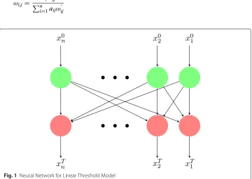
We build the Linear Threshold Neural Network (LTNN) shown in Fig.1to approximate the Linear Threshold Learning Model. The inputx0₁,x0₂,. . .,x0_nare the status ofnusers in social media networks at timet = 0. The output layer outputsxT₁,xT₂,. . .,xT_n, which are the status ofnusers in social media networks at timet=T.

There are several constraints to consider for the Linear Threshold Learning Model. Firstly, if the user is active in the beginning (xˆ0_j = 1), then they will stay active (xˆT_j = 1). To satisfy this constraint, we set the(i,j)entry of the neural network weights matrixW , denoted asw_i,j, as 1 wheniequalsj. In this case, when user is active at the beginning, the total influence it gets at timet = T will definitely be larger than its threshold and the user will stay active. Besides, the influence weights should be suppressed to 0 when the pair of users has no connection. Here, we use the Hadamard product of adjacency matrixAof the network and neural network weights matrixW to suppress the influence weights matrixW. Thirdly, in the Linear Threshold Model, the diffusion influence weights should be normalized as well. All of the constraints above could be satisfied by designing the structure of neural network. However, the Linear Threshold Model has the activation function of step function. The gradients of step function are vanishing and the weights will not update at all (Friesen and Domingos2017). The neural network is using gradient to update the estimation. Therefore, step function is not applicable to neural network. Instead, we approximate the step function using sigmoid function. Then the outputXT ₌

xT₁,xT₂,. . .,xT_n of neural network could be represented as: XT =Sigmoid

X0

(A+I)◦W

−θ

Whereθis the threshold vector of users andIis the identity matrix. As mentioned before, the influence weights are normalized as well, thus the diffusion influence weightωi,j(ωi,j∈

W)between useriand userjcould be represented as:

ωi,j=

aijω_{ij n}

i=1aijωij

Whereaijis the (i,j) entry of adjacency matrixAandω_ij is the (i,j) entry of artificial

neural network weights matrixW.

Artificial Neural Network for Random Walk Learning Model

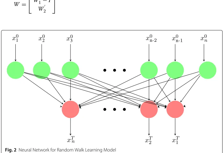
The structure of neural network called Random Walk Neural Network (RWNN) built for Random Walk Learning Model is shown in Fig.2. Here we consider the diffusion influence could be from 2-step neighborhood. Therefore, the input is the two times combination of the initial status ofnnodes, denoted asx0₁,. . .,x_n0,x0₁,. . .,x0_n. The output layer outputs xT₁,xT₂,. . .,xT_n, which are the status of users in the social media at timet=T.

To satisfy the constraints in Random Walk Learning Model, we make the following modifications to the artificial neural network. Considering the diffusion influence from two step neighborhood, the total influence shown in Eq.2in the Random Walk Model could be transferred as:

A1◦W1+A2◦W2

X0=X0 X0 A

1

A2

◦

W1

W2

Besides, the user will remain active when they are active in the beginning. Thus we add the identity matrixIto adjacency matrixAto satisfy the constraint. Then the output vector XT =xT₁,xT₂,. . .,xT_n of neural network could be represented as:

XT =SigmoidX0 X0 A

1_+I

A2

◦

W₁ W₂

−θ

Whereθis the threshold of users, A is the adjacency matrix,A2is the square of adjacency matrix.W₁andW₂are weights matrix of neural network. Thus the diffusion influence weights matrixWcould be represented as:

W =

W₁−I

W₂

Experimental Evaluation

In this section we conduct the experimental evaluation of our proposed models which are Linear Threshold Model, Random Walk Model, Linear Threshold Neural Network Model and Random Walk Neural Network Model to learn the information diffusion weights. We analyze the performance of proposed models on both synthetic data and real data.

Experiments on Synthetic Data

Firstly, we generate synthetic data to evaluate our models. The generation of synthetic data includes both network generation and cascade generation.

Network generation: In order to understand how the underlying network topol-ogy affects the performance of our learning models, we generate different well-known generative networks.

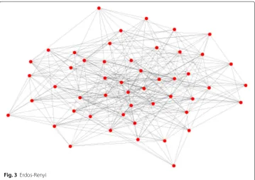
• Erdos-Renyi Graph:In the graph theory, Erdos-Renyi model generates random graph. Here we use theG(n,p)model in which a graph is constructed by connecting nodes randomly by edges with probabilityp. For experimental purpose, we generate the network shown in Fig.3containing 50 nodes and generate edges between each pair of nodes in the network with probability of 0.3.

• Barabasi-Albert Graph:Social media networks are thought to be scale-free. Barabasi-Albert graph generates random scale-free networks using a preferential attachment mechanism. Here we generate a graph of 50 nodes shown in Fig.4which is grown by attaching new nodes each with 15 edges that are preferentially attached to existing nodes with high degree.

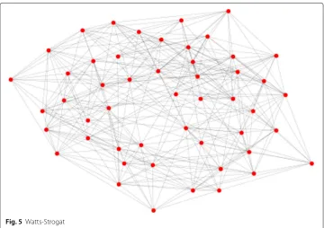
• Watts-Strogatz Graph:Watts-Strogatz model generates random graph with small-world properties, which are short average path lengths and high clustering. Here we generate a graph of 50 nodes shown in Fig.5, and each of them connects to 15 nearest neighbors. In addition, the probability of rewiring each edge is 0.5.

Fig. 4Barabasi-Albert

Cascade generation:We learn the diffusion influence weights from mining historical diffusion cascades. Here, we generate the cascades for the synthetic data. We randomly select a set of seed nodes accounting for 35% of total nodes . Then the seed nodes could propagate the information to other nodes. Here we assume the active nodes will remain active and the inactive nodes will have the chances to be activated only when they have connections to active nodes within 2 step neighborhood. The activation probabilitypfor target node is defined as:

p=a+ b

N ∗AN (4)

WhereNrepresents the total number of nodes andANrepresents the active direct neigh-bors. We setaas 0.5 andbas 0.5 for the following experiments. We experiment with 200 cascades to compare the performance of different learning models.

Implementation Details and Evaluation: In order to learn the diffusion influence weights under different proposed learning models, we set the threshold of 0.5 for each user in the social media network. In order to provide an unbiased evaluation of a final model on the training dataset, we split the dataset into training set and testing set with 80% of training set and 20% of testing set. To validate the performance of the mixed integer programming learning models and the approximate neural network learning models, we evaluate the performance of accuracy. Accuracy is the ratio of correct pre-dictions. Regarding to solve the problem using mixed-integer programming, we propose the decomposition method which is tractable to compute and to optimize for the origi-nal learning models. For each node, we apply the optimization model to get the diffusion weights separately because the diffusion influence from neighbors to each node is inde-pendent from each other. For the neural network learning models, we train in 10000 steps, with batch size of 10 and learning rate of 0.001.

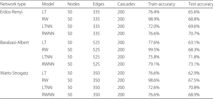
Experimental Results:For different network types, we generate the same number of cascades using the same cascade generation strategy to compare the performance of different models. Table1shows the performance of synthetic data of 50 nodes.

The performance of different learning models are consistent in different network topologies. For the same number of observations(cascades), approximate neural network learning methods even outperform the mixed integer programming learning methods. The mixed integer programming methods of Linear Threshold Model and Random Walk Model have severe overfitting problems. In addition, the computational time for mixed integer programming models is much longer than neural network based models.

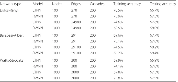
Therefore, for larger scale networks we conduct the experimental evaluation just using approximate neural network learning models. The performance of different sizes of net-works which are 100 nodes and 1000 nodes are shown in Table2. The testing accuracy is consistent for different network types.

Table 1Performance of synthetic data

Network type Model Nodes Edges Cascades Train accuracy Test accuracy

Erdos-Renyi LT 50 335 200 76.4% 65.6%

RW 50 335 200 98.9% 68.8%

LTNN 50 335 200 72.0% 69.6%

RWNN 50 335 200 76.6% 70.7%

Barabasi-Albert LT 50 525 200 77.6% 63.1%

RW 50 525 200 99.5% 68.3%

LTNN 50 525 200 75.8% 71.8%

RWNN 50 525 200 79.1% 73.1%

Watts-Strogatz LT 50 350 200 76.6% 62.9%

RW 50 350 200 98.6% 67.5%

LTNN 50 350 200 72.6% 70.8%

Table 2Performance of large-scale synthetic data

Network type Model Nodes Edges Cascades Training accuracy Testing accuracy

Erdos-Renyi LTNN 100 270 200 70.5% 66.7%

RWNN 100 270 200 73.9% 67.5%

LTNN 1000 24980 200 74.6% 67.6%

RWNN 1000 24980 200 68.5% 68.0%

Barabasi-Albert LTNN 100 291 200 69.6% 67.7%

RWNN 100 291 200 75.1% 67.0%

LTNN 1000 29100 200 74.5% 68.2%

RWNN 1000 29100 200 68.7% 68.4%

Watts-Strogatz LTNN 100 300 200 69.9% 66.9%

RWNN 100 300 200 74.1% 67.0%

LTNN 1000 3000 200 69.8% 67.5%

RWNN 1000 3000 200 73.8% 67.9%

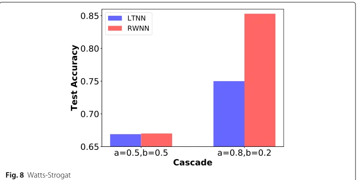
The performance of different models could be affected by the way of generating cas-cades. We test the performance of different generation methods by changingaandb parameters in Eq. 4 using the same network topology. The performance of different network topologies are shown in Figs. 6, 7and8. Whena is larger which means get-ting more influence from two step neighborhood, Random Walk Neural Network Model outperforms Linear Threshold Neural Network Model.

Experiments on Real Data

We collect the real data from Lerman Digg 2009 dataset (Lerman and Ghosh2010). The Digg 2009 dataset contains data about stories promoted to Digg’s front page over a period of a month in 2009. The dataset contains the time stamp of all of the users’ vote for the stories. Both of the network topology and cascade information can be obtained from the dataset.

Dataset Preprocessing:Considering the computation limitation of mixed integer pro-gramming models, we extract a small size subgraph containing 1203 nodes shown in Fig.9to compare the performance between mixed integer programming learning mod-els and approximate neural network learning modmod-els. Our extracted subgraph contains

Fig. 7Barabasi-Albert

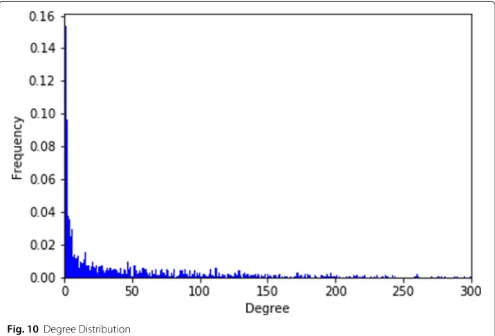
1203 users shown in Fig.9. In Fig.10, we could see the degree distribution of all the users follows power law distribution. The extracted network keeps the social network prop-erty of scale-free. In addition, to prove the effectiveness of the proposed models in large scale social network, we extract a network with 42259 nodes and conduct the experiments using neural network based models. In order to get the cascade information, we choose the most voted 600 stories. Then we collect all the users voting status at timeT0andTt

for each story.

Implementation Details and Evaluation:To investigate the performance on real data, we set the threshold of 0.5 for each user in each of the proposed learning models.

Experimental Results of Real Data:We proceed with experiments on preprocessed real data of 1203 nodes to see the performance of different learning models. We collect the historical cascades of 650 stories and get 406 efficient cascades. We treat 300 obser-vations as training samples and the rest of obserobser-vations as testing samples. For the neural network models, we train in 10000 steps with batch size of 10 and learning rate of 0.001. The performance of the dataset is shown in Table3. First, we evaluate the performance of different learning models based on test accuracy. Random walk learning model has the best performance in this preprocessed real dataset. It doesn’t have any overfitting issue

Fig. 9Network Topology

here which is likely due to the fact of sparseness of the network. In general, the ran-dom walk based learning models outperform the linear threshold based learning models in this preprocessed dataset. However, when it comes to the speed of computation, the approximate methods using neural network, i.e., LTNN and RWNN are much faster.

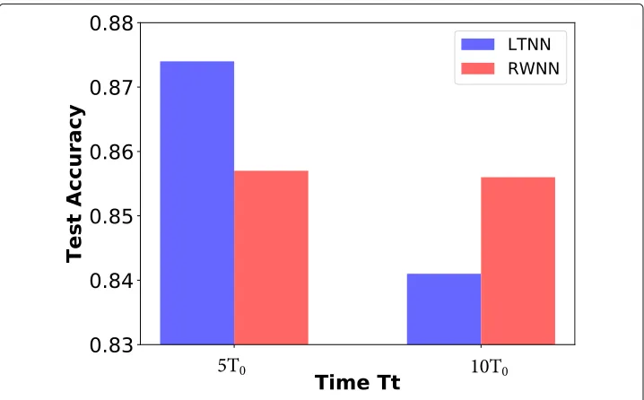
Then, we examine the performance of LTNN model and RWNN model using cascade information from different time intervals. We collect the data from different lengths of time intervals. One has the time interval of 4T0and another has the time interval of 9T0.

Table 3Performance of real data

Model Nodes Edges Cascades Training accuracy Testing accuracy Time(s)

LT 1203 29166 406 82.8% 86.3% 1773

RW 1203 29166 406 88.3% 92.3% 32406

LTNN 1203 29166 406 85.5% 84.1% 137

RWNN 1203 29166 406 86.4% 85.6% 330

Figure11shows the performance comparison of two approximate models during differ-ent time intervals. For shorter time period, the LTNN model has significant improvemdiffer-ent over RWNN model. In converse, RWNN model outperforms LTNN model in longer time period. This happens because in short time period, only one step propagation could hap-pen. In longer time period, two-steps or multiple steps propagation could occur where random walk based model would better describe the information diffusion process.

For the large scale network containing 42259 users, we collect the historical cascades of 600 stories and get 566 efficient casacades for experimental purpose. We treat 440 cascades as training samples and the rest as testing samples. We train in 500 steps with batch size of 10 and learning rate of 0.001. The cascade has the time interval of 9T0.

The experimental result of the large dataset is shown in Table4. Random Walk Neural Network Model requires 380GB memory and it takes about 10 min for each step. It’s time consuming and it gets stuck during the optimization process because of too many nodes. In comparison, Linear Threshold Neural Network Model converges in 500 steps and has very good performance.

Conclusions

We have investigated the problem of learning diffusion influence weights between pairs of users in social media networks from mining historical cascades. We formulate two dif-ferent mixed-integer programming models to learn the diffusion influence weights which

Table 4Performance of large-scale real data

Model Nodes Edges Cascades Training accuracy Testing accuracy Time(s)

LTNN 42259 1559768 566 91.2% 90.4% 22782

could be used to predict the status of users in the future. The first mixed integer program-ming model is based on the popular propagation model, i.e., Linear Threshold Model. The second mixed integer programming model is based on the idea of random walk considering the influence from multi-step neighborhood. For larger network, we intro-duce approximate approaches for both models using neural network. We bring marriage between optimization-based diffusion models and deep neural network through approx-imating optimization models using deep neural networks. Therefore, the parameters in the neural network are explainable, which are diffusion weights related parameters in our models. The approximate approaches using artificial neural networks have relatively good performance and fast computational speed.

There are several interesting directions for future works. Here we just learn the informa-tion diffusion influence through the historical cascades. It would be more interesting to consider other features such as the similarity between posters and reposters, the user pro-files or even the topology information of the social media networks to make predictions with higher accuracy.

Acknowledgements

This article is based on basic research works supported by AFRL Mathematical Modeling and Optimization Institute.

Authors’ contributions

ZQ proposed the approximate methods using neural network, implemented the experiments and analyzed the data. EP and QZ contributed to build optimization learning models. All authors read and approved the final manuscripts.

Funding

The research was funded by AFRL.

Availability of data and materials

Data is available on request from corresponding author.

Competing interests

The authors declare that they have no competing interests.

Author details

1_{Department of Industrial Engineering and Management Systems, University of Central Florida, Orlando 32826, FL, USA.} 2_{Air Force Research Laboratory, EglinAFB 32542, FL, USA.}

Received: 7 March 2019 Accepted: 20 September 2019

References

Avriel M (2003) Nonlinear programming: analysis and methods. Courier Corporation, Mineola Bishop CM (2006) Pattern recognition and machine learning. Springer, New York

Budak C, Agrawal D, El Abbadi A (2011) Limiting the spread of misinformation in social networks. In: Proceedings of the 20th International Conference on World Wide Web. ACM, New York. pp 665–674

Chen W, Lakshmanan LV, Castillo C (2013) Information and influence propagation in social networks. Synth Lect Data Manag 5(4):1–177

Domingos P (2005) Mining social networks for viral marketing. IEEE Intell Syst 20(1):80–82 Goodfellow I, Bengio Y, Courville A (2016) Deep learning. MIT press, Cambridge

Goyal A, Bonchi F, Lakshmanan LV (2010) Learning influence probabilities in social networks. In: Proceedings of the Third ACM International Conference on Web Search and Data Mining. ACM, New York. pp 241–250

Granovetter M (1978) Threshold models of collective behavior. Am J Sociol 83(6):1420–1443

Friesen AL, Domingos P (2017) Deep learning as a mixed convex-combinatorial optimization problem. arXiv preprint arXiv:1710.11573

Kimura M, Saito K, Motoda H (2009) Blocking links to minimize contamination spread in a social network. ACM Trans Knowl Disc Data (TKDD) 3(2):9

Kimura M, Saito K, Nakano R (2007) Extracting influential nodes for information diffusion on a social network. In: AAAI, vol. 7. AAAI Publication, Palo Alto, California. pp 1371–1376

Lerman K, Ghosh R (2010) Information contagion: An empirical study of the spread of news on digg and twitter social networks. In: Fourth International AAAI Conference on Weblogs and Social Media. AAAI Publication, Palo Alto, California

Rodriguez MG, Balduzzi D, Schölkopf B (2011) Uncovering the temporal dynamics of diffusion networks. arXiv preprint arXiv:1105.0697

Saito K, Kimura M, Ohara K, Motoda H (2009) Learning continuous-time information diffusion model for social behavioral data analysis. In: Asian Conference on Machine Learning. Springer, New York. pp 322–337

Saito K, Nakano R, Kimura M (2008) Prediction of information diffusion probabilities for independent cascade model. In: International Conference on Knowledge-Based and Intelligent Information and Engineering Systems. Springer, New York. pp 67–75

Publisher’s Note