Received June 16, 2010 Dongmin Kong ()
School of Economics, Huazhong University of Science and Technology, Wuhan 430074, China E-mail: kongdm@hust.edu.cn
Yuanyuan Shao
School of Economics, Huazhong University of Science and Technology, Wuhan 430074, China E-mail: shaoyy.happy@163.com
Jing Huang
School of Economics, Huazhong University of Science and Technology, Wuhan 430074, China E-mail: hj901103@gmail.com
RESEARCH ARTICLE
Dongmin Kong, Yuanyuan Shao, Jing Huang
Institutional Trading in IPOs and Post-IPOs:
Value-Based vs Speculative
© Higher Education Press and Springer-Verlag 2011
Abstract Using a unique dataset from Shanghai Stock Exchange, we study
institutional trading behaviors in IPOs and post-IPOs. From the perspective of value-based or speculation, we find that, (1) institutional investors are flippers on the first day of IPOs, (2) trading by institutional investors and the active institutional investors (mutual funds or brokerage) is value-based, and (3) the net buys of institutional investors can predict the long term performance of IPO-firms and shows a negative relation with a bubble in future. Since individual investors are the opponent of institutional investors, our results mean that individuals are speculators in the market. Our study suggest that institutional investors are the sophisticated ones in the market and they can process information more efficiently, whose value-based trading can enhance market price discovery and is good for market stabilization.
Keywords IPOs, institutional investor, trading behavior
1 Introduction
important role. Using a unique dataset from Shanghai Stock Exchange (SSE), we study institutions and active institutions’ trading behavior in IPOs and post-IPOs in terms of value-based or speculation.
Compared to the U.S. institutional investors, in an emerging market like China, institutional investors are still in an infant stage and mainly consist of mutual funds, whose behaviors are more often affected by the market status than those in the U.S. Therefore, is the trading behavior of institutional investors in IPOs and post-IPO value-oriented or speculative-oriented? Do institutional investors correct or amplify the pricing biases? What is the influence of institutional behaviors will have on the market stability and market efficiency? Answering these questions is important in practice and theory. Although related reports can often be found in media, there are rarely academic studies on these questions, especially in emerging markets.
Generally speaking, institutional investors, compared to individual investors, are always considered to have a greater ability to obtain and process information (e.g., Nagel, 2005; Cohen, Gompers et al., 2002; Badrinath, Kale and Noe, 1995; Michaely and Shaw, 1994). Therefore, we expect institutional investors’ trading in IPO and post-IPO will reflect the specific information superiority. Recently, Dor (2004) and Field and Lowry (2009) find that IPO firms with higher institutional shareholdings outperform those with lower institutional shareholdings, and Field and Lowry (2009) further point out that the difference in their performances is 13.2% in respect of one year holding period. The underlying reason of the difference is that IPO firms with lower institutional holdings have extremely low abnormal return, as compared with the high abnormal returns of IPO firms with higher institutional holdings.
A natural follow-up question is that how can institutional investors identify or avoid stocks with poor performance? Chemmanur, He and Hu (2009) find that institutional investors have private information, which brings them abnormal return from SEO. Chemmanur and Hu (2009) also find that institutional investors in post-IPOs can get abnormal return for several months based on private information. Boehmer, Boehmer and Fishe (2006) also believe that institutional investors have the ability to obtain better IPOs allocations and private information, which helps institutional investor to beat the market. All of these studies argue that what account for the abnormal return of institutional investors is that they have private information.
From another point of view, institutional investors in IPOs may not have any information. The motivation of transactions comes from their market advantage, e.g., institutions have the ability to create a certain price tendency to attract other investors into the market and buy or sell when the price reaches a certain shape to get profit. This can be seen as a price manipulation to some degree. Boehmer, Boehmer, and Fishe (2006) find that institutional investors don’t sell the stocks with poor future performance immediately, which means that institutions do not have information superiority.
To the best of our knowledge, there is no study giving direct evidences on institutions’ (active/passive) and individuals’ trading in IPOs and post-IPOs, or study on whether institutional investors’ trading in IPOs and post-IPOs can predict the company‘s long-term performance. We fill the gap in this paper. Besides, we also study the relation between trading behavior and other variables which is also showed in Green and Hwang (2009) and Kumar (2009), such as the IPO-firms’ future performance, stock price bubbles and so on.
The rest of the paper is organized as follows: Section 2 discusses the related literature, Section 3 proposes the construction of hypotheses, Section 4 describes data and methodology, Section 5 presents empirical results, and we conclude in Section 6.
2 Literature Review
Aggarwal (2003) studies IPOs allocation and flipping over the first two days after the IPOs. Boehmer, Boehmer and Fiche (2006) study the relations between IPO allocation, flipping, and long-run IPO performance. Bayley, Lee and Walter (2006) study the flipping activities in Australian IPOs. Ellis, Michaely and O’Hara (2000) and Ellis (2006) study the trading behavior of market makers in the IPOs aftermarket. Overall, these papers focus on flipping or trading behavior in the immediate post-IPOs period.
However, in this paper, we study the institutional investors’ trading in IPOs and post-IPOs, and relations between trading behavior and future company performance, stock price bubble and so on. Based on these relations, we can further study whether the differences in different investors’ trading exist and how these behaviors affect market efficiency.
predictability. Our results on the predictive power of the first two days of institutional trading are consistent with those. However, there are important differences between our study and related research. We extend in several directions, such as institutions’ long-run predictability, the participation of institutions in speculative stocks and institutions’ ability to forecast future stock price bubbles.
In addition to studying institutional investors’ trading behavior in IPOs, we also study the investors’ ability to predict the performance of the first following year by researching their behavior during a period after IPOs and distinguish the behavioral differences between different institutional investors. Further, our data advantage (the data based on account-level of the transaction records of all investors in market, while other studies just use a subset of all transactions/ investors) can ensure complete information. Then we can further infer the individual investors’ behaviors through trading by the institutional (Obviously, it is impossible to infer the other type investors’ behaviors only using a subset of the whole transaction in market).
Additionally, Krigman, Shaw, and Womack (1999) study institutional flipping by identifying block sale in the TAQ data, which means they cannot really identify institutional or individual investors’ trading. These studies often use the size of each transaction to classify investors. If the transaction volume is large, the transaction is defined as the institutions’ trading, and if its volume is small, it will be defined as individual investors’ trading. It is well known that the algorithm for judging the direction of trade, while useful, is far from being perfect. This algorithm has two obvious drawbacks: First, deviations in the classification of transactions must exist; second, the approach cannot be used to infer the investors with medium-sized transactions, which will obviously lead to the loss of information.
Different from Krigman, Shaw and Womack’s (1999) focusing on flipping alone, we study institutional net buying (buying minus selling) in IPOs, and thus provide a more complete picture. We also study this from the perspective of investor preferences in speculation, which is also showed in other researches, such as Green and Hwang (2009) find that stocks with high expected skewness has a higher rate of return on the first day and Kumar (2009) which find that individual investors in IPOs have more preference in lottery.
Almost all of the IPOs research in China focuses on the IPO underpricing and the long-term performance, there’s no study which is from the point of the institutional investors’ trading behavior.
3 Hypotheses
prevalent phenomenon in the capital market, which is the so-called “money left on the table.” For institutional investors, in order to get the money left on the table, they would likely sell shares bought in IPOs on the offering day in the secondary market. There are many studies about institutional investors’ flipping activity, such as Aggarwal (2003), Boehmer, Boehmer and Fishe (2006), Bayley, Lee and Walter (2006), Ellis, Michaely, and O’Hara (2000) and Ellis (2006). However, these studies do not use the account level data like our paper does. So we propose the “flipping” hypothesis:
H1 On the first day of trading, the behavior of institutional investors is a significant net selling (the behavior of individual investors behavior is a significant net buying).
A straightforward way to determine the trading behavior of institutional investors is value-based or speculative and whether the institutional investors are sophisticated on information processing or not is to examine the relationship between institutional investors trading and future performance of IPOs. As compared to individual investors, institutional investors can obtain more information, so we can assume that the more rational institutional investors is value-based, who will make full use of the information possessed and make appropriate assessment about the company’s future prospects and of performance.
From the perspective of long-term investment, investing the stocks which will have good prospects is undoubtedly beneficial for investors. Thus, if institutional investors in IPOs and post-IPOs can predict the future performance of stocks, they will hold more stocks which perform better in future. This point is similar to the conclusion of Chemmanur, He and Hu (2009), which find that, in SEOs, the buying behaviors of institutional investors is positively related to firms’ future performance. Our second hypothesis is as follows,
H2 In IPOs and post-IPOs, the stocks which have more net buying by institutional investors in early post-offering days have better long-term performance.
Generally speaking, institutional investors are more rational. For rational agents in the market, they probably consider that stocks with higher issue price in IPOs have bigger bubbles, and thus, these stocks face larger risk in the future. Based on this argument, we speculate that rational institutional investors prefer the relative lower-price (e.g., price-earnings ratio) stocks. We have the following hypothesis:
Green and Hwang (2009) suggest that individual investors tend to buy stocks with high skewness in IPOs. They argue the pricing skewness of IPO stocks is the proxy for speculation and stocks with higher expected skewness have higher return on the first day of IPOs. Furthermore, they find that stocks with high skewness are often shifted from institutional investors to individual investors, which indicates that individual investors prefer stocks with speculative characteristics. Kumar (2009) also point out that those stocks with low price, large skewness and high volatility are speculative stocks. Thus, if institutional investors are value-based, they will buy fewer speculative stocks and individual investors will have a larger net buying on speculative shares. We get the following hypothesis,
H4a In IPOs and post-IPOs, the more speculative stocks are, the less institutional investors buy.
However, an alternative argument, especially in the China’s stock market, is that institutional investors can create a “bubble” to attract other investors to enter, then institutions take the opportunity to withdraw (which is called “pump and dump” commonly found in documents), so we can also suppose that most of informed traders are institutional investors (which is in line with intuition). If this argument is true, the net buying of institutional investors may show a positive relationship with the stock speculative grade. Accordingly, we propose the competitive hypothesis of H4a:
H4b In IPOs and post-IPOs, the more speculative stocks are, the more institutional investors buy.
Furthermore, if institutional investors indeed have more information about the IPOs or they have more inference skills than individual investors, we speculate that the institutional should know more about the true value of stocks, which can help them to judge the firm’s prospect or predict future trends of the stocks more precisely. It is reasonable for us to believe that the future stock bubbles will affect the institutional investors’ trading behavior. Thus, the stocks largely bought by institutional investors would have less speculative bubbles in the future. Accordingly, our H5 is as follows,
H5 In IPOs and post-IPOs, institutional investors show lower level of net buying to the IPOs with higher future stock bubbles.
4 Data and Methodology
4.1 Data Sources1, 2005 and December 31, 2007. The net buying (NB) data of institutions, active institutions, and individuals were computed from account level data from “Financial Innovation Research Lab” in Shanghai Stock Exchange.1 With this dataset, we can identify the types of investors according to the account types precisely. Other relative data were obtained from the SinoFin database. There were altogether 41 IPOs during our sample period.
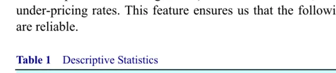
The basic statistical distributions of sample data are illustrated in Table 1. According to the results, the sample companies exhibit reasonable variability (i.e., our samples are heterogeneous) in market values, IPO P/E ratios, and under-pricing rates. This feature ensures us that the following regression results are reliable.
Table 1 Descriptive Statistics
Variables Obs. Mean S.D. Min Max Median
Market value (Million Yuan) 41 13 231 177 300 66 800 6 201
IPO P/E ratio 40 29.696 20.705 7.500 98.67 24.085
Demand to offer ratio (%) 39 1.035 3 1.041 1 0.063 3 5.33 0.617
Under-pricing ratio (%) 41 95.84 84.93 0 424.00 71.70
4.2 Methodology
Our key variable for investors’ trading behavior, net buying (NB), is calculated as follows:
,
i,t i,t i, j
i,t i,t
Buy Sell NB =
Buy + Sell
−
(1)
where NBi,j is the net buying of the ith type of investors (institutional investors,
active institutions and individual investors) on the jth day. Buyi,t is the total
buying of the ith type of investors on the tth day and Selli,t is the total selling of
the ith type of investors on the tth day. In the following statistical tests we focus
on trading by institutional and active institutions, based on which the behavior of individual investors can be inferred, since our data is the whole market trading records (the sum of transactions of institutional investors and individual investors is definitely the whole market transactions).
To test H1, we directly examine the behavior of institutional investors on the first day of IPOs. Specifically, using t-test based on one sample, we examine
1 The original dataset of trading accounts exceeds hundreds of Gigabytes in size and includes
whether the net buying of institutional (and active institutional) investors are significantly negative, i.e., whether the flipping activities of these investors are significant. Of course, we can infer the net buying of individual investors from this.
For H2, we examine the relationship between the behaviors of institutional investors in the 30-trading days of post-IPOs and the long-run performance of these listed companies. We adopt a regression model as follows:
1 1 ,
i,T year j j
j
NB = a + b Perf +
∑
d Control_Variables + e (2)where NBi,T is the net buying of the ith type of investors (institutional investors,
active institutions and individual investors) in the period of T of post-IPOs.
Perfyear1is the long-run performance of the listed companies and for proxies we
choose ROE and Tobin’s Q in the first year after offering. Control_Variables are controlling variables chosen following the pattern of former researchers, including Ln(Size): the log size of listed companies’ market values; Age: the time interval (years) between the establishment of the company and its offering day;
DO_Ratio: the demand to offer ratio of IPOs; Gap: the time (days) IPOs have been listed; and Underwriter: dummy variable measuring the reputation of lead underwriter-equals one if it is in top ten of underwriters according to the market share order and equals zero if it is not.
H3 examines the influences of issuing prices on investors’ behaviors in a short time after IPOs. We assume that the net buying of institutional investors decreases as the issuing price of that IPO increases. We exclude the net buying of investors on the first day of IPOs, since we examine the flipping activities in H1. Specifically, we introduce a regression model as follows:
1 ,
i,T j j
j
NB = a + b IssuePrice +
∑
d Control_Variables + e (3)where NBi,T is the net buying of the ith type of investors (institutional investors,
active institutions and individual investors) in the period of T of post-IPOs.
IssuePrice is issue price of stock on the offering day; Control_Variables are controlling variables the same as those defined above.
Since the stock price only measures the absolute price, we also include a price relative to the company’s earnings (based on P/E ratio) to study the relationship between investor’s behavior and this relative price-APE (Abnormal P/E ratio of listed company). The way to calculate APE of a certain IPO-stock is as follows:
(
j j)
,j
IPE =
∑
w ×PE (4)where PE j is the jth stock’s P/E ratio and w j is the weight of market share of the
jth stock in the industry. APE is then calculated as:
.
IssuePE IPE APE
IPE
−
= (5)
Thus, an alternative regression model of equation (3) is:
1 .
i,T j j
j
NB = a + b APE +
∑
d Control_Variables + e (6)H4 examines investor’s preference for speculative stocks. Using a stock’s skewness as proxy for speculative grade, we adopt the following model to examine the relationship between investors’ behaviors in early post-offering days and speculative grade of IPOs.
1 ,
i,T j j
j
NB = a + b Skewness +
∑
d Control_Variables + e (7)where NBi,T is the net buying of the ith type of investors (institutional investors,
active institutions and individual investors) in the period of T of post-IPOs. Skewness is the skewness of a listed company’s stock and is a proxy for its speculative level. According to the percentile approach in Green and Hwang (2009), a certain IPOs’ expected skewness is measured by skewness of stocks in the same industry:
99 50 50 1
99 1
( ) ( )
,
P P P P
Skewness
P P
− − −
=
− (8)
where Pj is the jth percentile of the log return distribution pooled across all stocks
within the CSRC-industry of IPO i over 60 trading days of the offering. If the right tail is further away from the median than is the left tail, realizations of Skewness are positive, indicating that the distribution is right skewed. According to Green and Hwang (2009), this approach properly captures the notion that skewness-preferring investors may care about the tail events when judging a stock’s lottery-like return distribution as opposed to the entire distribution.
Control_Variables are controlling variables the same as those defined above. H5 concerns whether the institutional investors can recognize the bubbles in future stock’s price. The regression model is set by including the P/E ratio in the first year after the offering:
1 1 ,
i,T year j j
j
NB = a + b PE +
∑
d Control_Variables + e (9)where P/Eyear1 is the PE ratio of the first year after the offering and
5 Results
5.1 Summary Statistics
Table 2 reports the trading behaviors of different types of investors during different time period after the offering. We find that institutional investors are net sellers of IPOs on the offering day, which means significant flipping activities, while in the following one to two weeks institutional investors show a pattern of net buying. From two weeks to one month after the offering, a certain degree of net selling is presented.
Table 2 Net Buying of Institutional Investors and Active Institutional Investors
Institutional investors
(opposite to individuals) Active institutional investors (mutual funds or brokerages) Interval Obs.
Mean S.D. Min Max Mean S.D. Min Max
[T1] 41 –0.056 1 0.107 1 –0.270 8 0.272 4 0.011 6 0.070 2 –0.087 0 0.285 7
[T2,T6] 40 0.000 0 0.046 7 –0.183 8 0.134 5 0.008 2 0.029 5 –0.022 8 0.117 7
[T2,T11] 40 0.006 3 0.061 9 –0.211 0 0.196 6 0.014 7 0.041 2 –0.027 4 0.173 2
[T5,T11] 39 0.008 0 0.034 6 –0.078 6 0.112 7 0.009 8 0.026 1 –0.015 9 0.108 4
[T2,T21] 40 0.003 5 0.061 0 –0.200 6 0.200 0 0.017 4 0.043 6 –0.038 3 0.187 6
[T2,T31] 40 0.001 5 0.086 2 –0.221 7 0.329 3 0.018 4 0.049 5 –0.050 2 0.184 1
[T5,T21] 39 0.005 1 0.037 9 –0.063 1 0.116 1 0.012 4 0.030 6 –0.031 6 0.122 8
[T5,T31] 39 0.003 1 0.074 7 –0.221 2 0.318 7 0.013 6 0.039 5 –0.066 3 0.166 4
[T10,T21] 37 –0.000 6 0.033 9 –0.085 2 0.123 2 0.005 5 0.024 1 –0.027 0 0.103 4 [T10,T31] 37 –0.002 8 0.075 2 –0.229 7 0.326 3 0.006 7 0.036 9 –0.093 8 0.175 4 [T20,T31] 35 –0.001 8 0.051 2 –0.163 8 0.214 8 0.002 2 0.020 7 –0.071 0 0.083 7
Note: This table reports the net buying of institutional investors (opposite to the trading behavior of individuals) and active institutional investors (mutual funds, brokerages etc.) during respective time period in the early post-offering days. The intervals here represent different statistical time periods, where the microscopic number i beside T represent the ith trading day
after the offering. The variable NB is calculated according to Equation (1).
5.2 Findings
To directly test whether institutional investors are significant net sellers of IPOs on the offering day (H1), we depict the histograms (Fig. 1) of institutional investor’s net buying on the offering day. NB of institutional investors is illustrated in the left sub-figure, which depicts that most of institutional investors are net sellers, indicating that individual investors are the net buyers of IPOs because their trading behavior is opposite to institutional investors’.
The sub-figure on the right illustrates net buying of active institutions which include mutual funds and brokerages. As depicted, except for two outliers on the right, active institutions do not show significant net selling and the mean value of
NB is distributed around zero.
Results of t-test in Table 3 further confirm our assumption: the net buying of individual investors is significantly negative and the null hypothesis is rejected on a significance level of 0.01, thereby proving institutional investors on the whole present significant net selling of IPOs on the offering day. The purpose of net selling is probably to get the “money left on the table” with the under pricing of IPOs. In the mean time, NB of active institutions is not significant and there is no styled pattern for their trading behavior in the first day of IPOs.
Fig. 1 Distributions of Institutional Investors’ Net Buying on the First Days of IPOs
Table 3 t-Test of Trading Behavior of Institutional Investors on the Offering Day
Types Obs. Mean t-value p-value
Institutions investors
(opposite to individuals) 41 –0.056 1 –3.357 3
*** 0.000 9
Active Institutions investors
(mutual funds or brokerage) 41 0.011 6 1.060 9 0.152 4
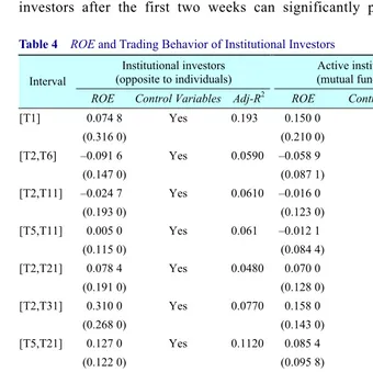
in early post-IPOs can predict long-run performance. Results are reported in Table 4. We find that in the following few days of IPOs, the results don’t show a clear relation between net buying of institutional investors and long-run performance of IPO-firms. However, the trading behavior of institutional investors after the first two weeks can significantly predict the long-run
Table 4 ROE and Trading Behavior of Institutional Investors
Institutional investors (opposite to individuals)
Active institutional investors (mutual funds or brokerages) Interval
ROE Control Variables Adj-R2 ROE Control Variables Adj-R2
[T1] 0.074 8 Yes 0.193 0.150 0 Yes 0.173
(0.316 0) (0.210 0)
[T2,T6] –0.091 6 Yes 0.0590 –0.058 9 Yes 0.168 0
(0.147 0) (0.087 1)
[T2,T11] –0.024 7 Yes 0.0610 –0.016 0 Yes 0.152 0
(0.193 0) (0.123 0)
[T5,T11] 0.005 0 Yes 0.061 –0.012 1 Yes 0.126 0
(0.115 0) (0.084 4)
[T2,T21] 0.078 4 Yes 0.0480 0.070 0 Yes 0.177 0
(0.191 0) (0.128 0)
[T2,T31] 0.310 0 Yes 0.0770 0.158 0 Yes 0.203 0
(0.268 0) (0.143 0)
[T5,T21] 0.127 0 Yes 0.1120 0.085 4 Yes 0.181 0
(0.122 0) (0.095 8)
[T5,T31] 0.385 0 Yes 0.1380 0.185 0 Yes 0.218 0
(0.240 0) (0.121 0)
[T10,T21] 0.162 0 Yes 0.1970 0.141* Yes 0.200 0
(0.112 0) (0.079 5)
[T10,T31] 0.441* Yes 0.1740 0.248** Yes 0.243 0
(0.252 0) (0.118 0)
[T20,T31] 0.363* Yes 0.2120 0.146* Yes 0.235 0
(0.182 0) (0.072 7)
Note: This table presents the regression results of Equation (2). ROE is return on equities in the first cohort year. Control Variables include: Ln(Size), the log size of listed companies’ market values; Age, the time interval (years) between the establishment of the company and the offering day; DO_Ratio,the demand to offer ratio of IPOs; Gap, the time interval (days) IPOs have been listed; Underwriter: dummy variable measuring the reputation of lead underwriter-equals one if the lead underwriter is in top ten of underwriters according to the market share order and equals zero if it is not. We use different NB as dependent variable in different time periods. Adj-R2is adjusted R-square. Robust Standard Errors are reported in
performance of the new listed companies. For example, with other factors controlled, the null hypothesis that trading behavior of institutional investors during [T10, T31] and [T20, T31] is uncorrelated with long-run performance (ROE) is significantly rejected.
It is reasonable to think that the trading behavior of institutional investors after some days of IPOs is related to the long-run performance of listed companies, and this result means institutional investors can make better prediction than individual investors. Limited by space and our focuses, we omit coefficients and standard errors of control variables, but these results are available upon e-mail.
For active institutions (such as mutual funds), we also get similar but more significant results, which confirm that trading behavior of active institutions after some days of the offering can significantly predict long-run performance of listed companies as well. Moreover, it is easy to infer that trading behavior of individual investors is negatively related to the long-run performance of listed companies so their trading behavior does not appear to be value-based.
In addition, we also test the correlation between Tobin’s Q in the first year after IPOs and investors’ trading behavior in the early post-offering days. Although their trading behavior is not significantly correlated with Tobin’s Q, the coefficients are positive with p-values near 10% significance level. This is probably because of the small observation of sample data (29 of the 41 IPOs are left when financial listed companies are excluded). Statistical results of active institutions are similar: positive coefficients and p values near 10% significance level.
Thus, as a whole, we conclude that institutional and active institutions can predict the long-run performance of IPO firms (one or two weeks after the offering). They adjust trading behavior based on such predictions as they can generally be right. Based on these results, we conclude that trading behaviors of institutional and active institutions are value-based while those of individual investors are not.
Statistical results related to H3 are presented in Table 5 and Table 6. From Table 5, institutional and active institutions share the same feature that NB coefficients are negative in a short time after the offering but gradually turn positive as time goes by. This means in the early post-offering days, institutional investors mainly sell IPOs with high absolute prices, probably because the prices are abnormally high and such stocks are correlated with more “money left on the table,” thus incurring more intense flipping activities. Although sharing a similar pattern, institutional investors as a whole show significant net sell in the early post-offering days while active institutions only show significant net buy in the days after that.
speculative stocks, institutional investors tend to sell out IPOs with high issue price. However, their trading behavior changes in later days might because they consider other fundamental factors of these listed companies.
The results might be biased since Table 5 is only based on absolute price which doesn’t reflect the earning of listed companies. We then use APE as a proxy for issue price and the results are presented in Table 6.
Table 5 Issue Price and Trading Behavior of Institutional Investors
Institutional investors
(opposite to individuals) Active institutional investors (mutual funds or brokerages) Interval
Issue price Control variables Adj-R2 Issue price Control variables Adj-R2
[T2,T6] –0.003 3*** Yes 0.2580 –0.000 4 Yes 0.163 0
(0.001 1) (0.000 7)
[T2,T11] –0.003 6** Yes 0.2080 0.000 0 Yes 0.152 0
(0.001 5) (0.001 0)
[T5,T11] –0.001 2 Yes 0.1070 0.000 4 Yes 0.132 0
(0.000 9) (0.000 7)
[T2,T21] –0.003 0* Yes 0.1440 0.000 8 Yes 0.182 0
(0.001 5) (0.001 1)
[T2,T31] –0.002 5 Yes 0.0740 0.001 3 Yes 0.201 0
(0.002 3) (0.001 2)
[T5,T21] –0.000 5 Yes 0.0870 0.001 3 Yes 0.225 0
(0.001 0) (0.000 8)
[T5,T31] 0.000 1 Yes 0.0670 0.001 9* Yes 0.243 0
(0.002 1) (0.001 0)
[T10,T21] 0.000 5 Yes 0.1480 0.001 1* Yes 0.193 0
(0.000 9) (0.000 6)
[T10,T31] 0.001 1 Yes 0.0950 0.001 7* Yes 0.209 0
(0.002 1) (0.001 0)
[T20,T31] 0.000 8 Yes 0.1060 0.000 8 Yes 0.180 0
(0.001 5) (0.000 6)
Note: This table presents the regression results of Equation (3). IssuePrice is the issuing price of IPOs on the offering day. Control Variables include: Ln(Size), the log size of listed companies’ market values; Age, the time interval (years) between the establishment of the company and the offering day; DO_Ratio, the demand to offer ratio of IPOs; Gap, the time interval (days) IPOs have been listed; Underwriter: dummy variable measuring the reputation of lead underwriter-equals one if the lead underwriter is in top ten of underwriters according to the market share order and equals zero if it is not. We use different NB as dependent variable in different time periods. Adj-R2is adjusted R-square. Robust Standard Errors are
Table 6 APE and trading behavior of institutional investors
Institutional investors (opposite to individuals)
Active institutional investors (mutual funds or brokerages) Interval
APE Control variables Adj-R2 APE Control variables Adj-R2
[T2,T6] –0.032 1 Yes 0.072 0 –0.012 3 Yes 0.178 0
(0.029 4) (0.016 4)
[T2,T11] –0.037 7 Yes 0.079 0 –0.007 98 Yes 0.143 0
(0.036 0) (0.021 7)
[T5,T11] –0.011 1 Yes 0.071 0 0.003 44 Yes 0.094 0
(0.018 6) (0.014 2)
[T2,T21] –0.065 3* Yes 0.145 0 –0.024 7 Yes 0.177 0
(0.034 4) (0.021 0)
[T2,T31] –0.110** Yes 0.180 0 –0.037 8 Yes 0.208 0
(0.051 4) (0.027 1)
[T5,T21] –0.038 8* Yes 0.210 0 –0.013 3 Yes 0.140 0
(0.021 0) (0.015 5)
[T5,T31] –0.083 3* Yes 0.185 0 –0.026 4 Yes 0.176 0
(0.046 1) (0.023 9)
[T10,T21] –0.034 1 Yes 0.238 0 –0.020 6 Yes 0.207 0
(0.022 6) (0.014 3)
[T10,T31] –0.082 4 Yes 0.182 0 –0.035 7 Yes 0.200 0
(0.051 1) (0.025 1)
[T20,T31] –0.054 7 Yes 0.205 0 –0.019 3 Yes 0.205 0
(0.034 2) (0.014 4)
Note: This table presents the regression results of Equation (6). APE is the abnormal P/E ratio of listed companies. Control Variables include: Ln(Size), the log size of listed companies’ market values; Age, the time interval (years) between the establishment of the company and the offering day; DO_Ratio, the demand to offer ratio of IPOs; Gap, the time interval (days) IPOs have been listed; Underwriter: dummy variable measuring the reputation of lead underwriter-equals one if the lead underwriter is in top ten of underwriters according to the market share order and equals zero if it is not. We use different NB as dependent variable in different time periods. Adj-R2is adjusted R-square. Robust Standard Errors are reported in
parentheses. *, ** and *** respectively denotes significance level of 0.10, 0.05 and 0.01.
investors of sample period is value-based. Coefficients relevant to active institutions are not significant but these negative coefficients at least do not prove them (i.e., mutual funds, brokerages, etc) to be the speculative.
Table 7 Skewness andTrading Behavior of Institutional Investors
Institutional investors (opposite to individuals)
Active institutional investors (mutual funds or brokerages) Interval
Skewness Control_variables Adj-R2 Skewness Control_variables Adj-R2
[T1] –0.109 Yes 0.232 0.002 0 Yes 0.207
(0.084 4) (0.243)
[T2,T6] 0.006 0 Yes 0.048 –0.056 7 Yes 0.175
(0.040 3) (0.102)
[T2,T11] –0.003 6 Yes 0.061 –0.006 0 Yes 0.176
(0.052 8) (0.143)
[T5,T11] –0.009 56 Yes 0.064 0.036 7 Yes 0.144
(0.029 6) (0.092 7)
[T2,T21] –0.022 2 Yes 0.095 0.066 9 Yes 0.203
(0.031 9) (0.105)
[T2,T31] –0.016 5 Yes 0.046 0.024 6 Yes 0.213
(0.052 3) (0.148)
[T5,T21] –0.050 7 Yes 0.052 –0.007 9 Yes 0.233
(0.074 2) (0.165)
[T2,T31] –0.057 0 Yes 0.090 0.034 1 Yes 0.216
(0.063 8) (0.134)
[T10,T21] –0.012 4 Yes 0.145 0.026 2 Yes 0.133
(0.028 9) (0.088 3)
[T10,T31] –0.050 4 Yes 0.105 –0.013 4 Yes 0.164
(0.065 6) (0.133)
[T20,T31] –0.035 Yes 0.116 –0.051 0 Yes 0.153
(0.044 9) (0.079 3)
Note: This table illustrates the results of regression equation (7). Skewness is the proxy for speculative level of IPOs. Control Variables include: Ln(Size), the log size of listed companies’ market values; Age, the time interval (years) between the establishment of the company and the offering day; DO_Ratio,the demand to offer ratio of IPOs; Gap, the time interval (days) IPOs have been listed; Underwriter: dummy variable measuring the reputation of lead underwriter-equals one if the lead underwriter is in top ten of underwriters according to the market share order and equals zero if it is not. We use different NB as dependent variable in different time periods. Adj-R2is adjusted R-square. Robust Standard
Test for H4 is shown in Table 7. According to the table, the results are very ambiguous. What results in this may be the duality of the H4, that is, H4a and the completive H4b may affect each other. So we can get a clear conclusion from the result. Generally, the regression coefficients of the institutions are negative, which might suggest that institutional investors prefer the stocks with lower speculation, while active institutions’ regression coefficients are positive, which might mean active institutions like to participate in speculative stocks in short period to follow market tendency. However, we cannot draw any statistically significant conclusions.
According to the results of Table 7, at least we cannot get any evidence to prove that institutions and active institutions prefer the speculative stocks. In addition, we cannot confirm the method to use the skewness as the proxy for the speculation, which may also have affected our test results.
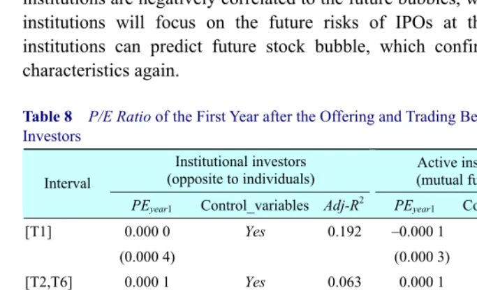
Finally, we examine the H5 which assumes that whether the different types of investors have the ability to predict future stock price bubble. As shown in Table 8, during post-offering days, the trading behavior of both institutions and active institutions are negatively correlated to the future bubbles, which also means that institutions will focus on the future risks of IPOs at that time. Therefore, institutions can predict future stock bubble, which confirms the value-based characteristics again.
Table 8 P/E Ratio of the First Year after the Offering and Trading Behavior of Institutional Investors
Institutional investors
(opposite to individuals) (mutual funds or brokerages) Active institutional investors Interval
PEyear1 Control_variables Adj-R2 PEyear1 Control_variables Adj-R2
[T1] 0.000 0 Yes 0.192 –0.000 1 Yes 0.162
(0.000 4) (0.000 3)
[T2,T6] 0.000 1 Yes 0.063 0.000 1 Yes 0.174
(0.000 2) (0.000 1)
[T2,T11] 0.000 0 Yes 0.060 0.000 0 Yes 0.152
(0.000 2) (0.000 1)
[T5,T11] –0.000 1 Yes 0.068 0.000 0 Yes 0.129
(0.000 1) (0.000 1)
[T2,T21] –0.000 1 Yes 0.054 –0.000 1 Yes 0.177
(0.000 2) (0.000 2)
[T2,T31] –0.000 5 Yes 0.106 –0.000 2 Yes 0.223
(0.000 3) (0.000 2)
(Continued)
Institutional investors (opposite to individuals)
Active institutional investors (mutual funds or brokerages) Interval
PEyear1 Control_variables Adj-R2 PEyear1 Control_variables Adj-R2
[T5,T21] –0.000 2 Yes 0.144 –0.000 1 Yes 0.197
(0.000 1) (0.000 1)
[T2,T31] –0.000 55** Yes 0.185 –0.000 29** Yes 0.273
(0.000 3) (0.000 1)
[T10,T21] –0.000 2 Yes 0.202 –0.000 1 Yes 0.179
(0.000 1) (0.000 1)
[T2,T31] –0.000 54* Yes 0.199 –0.000 30** Yes 0.268
(0.000 3) (0.000 1)
[T20,T31] –0.000 85*** Yes 0.408 –0.000 38*** Yes 0.503
(0.000 2) (0.000 1)
Note: This table presents the regression results of Equation (9). PEyear1 is P/E ratio in the first cohort
year of IPOs. Control Variables include: Ln(Size), the log size of listed companies’ market values; Age, the time interval (years) between the establishment of the company and the offering day; DO_Ratio,the demand to offer ratio of IPOs; Gap, the time interval (days) IPOs have been listed; Underwriter: dummy variable measuring the reputation of lead underwriter-equals one if the lead underwriter is in top ten of underwriters according to the market share order and equals zero if it is not. We use different NB as dependent variable in different time periods. Adj-R2is adjusted R-square. Robust Standard Errors are reported in
parentheses. *, ** and *** respectively denotes significance level of 0.10, 0.05 and 0.01.
6 Conclusion
Based on a unique dataset from SSE, we study the different types of investors’ (institutions, individuals and active institutions) trading behavior in IPOs.
Acknowledgements This work is supported by the National Natural Science Foundation of China (No. 70803013). We gratefully acknowledge the help from Donghui Shi, Di Liu, and Weidong Zhang of the Research Center of Shanghai Stock Exchange.
References
Aggarwal, R. 2003. Allocation of initial public offerings and flipping activity. Journal of Financial Economics, 68(1): 111–135.
Badrinath, S., Kale, J., & Noe, T. 1995. Of shepherds, sheep, and the cross-autocorrelations in equity returns.Review of Financial Studies, 8(2): 401–430.
Bayley, L., Lee, P. J., & Walter, T. S. 2006. IPO flipping in Australia: cross-sectional explanations. Pacific-Basin Finance Journal, 14(4): 327–348.
Boehmer, B., Boehmer, E., & Fishe, R. P. H. 2006. Do institutions receive favorable allocations in IPOs with better long-run returns? Journal of Financial and Quantitative Analysis, 41(4): 809–828.
Chemmanur, T., He, S., & Hu, G. 2009. The role of institutional investors in seasoned equity offerings. Journal of Financial Economics, 94: 384–411.
Chemmanur, T., & Hu, G. 2009. The role of institutional investors in initial public offerings. Working paper.
Cohen, R. B., Gompers, P. A., & Vuolteenaho, T. 2002. Who underreacts to cash-flow news? Evidence from trading between individuals and institutions. Journal of Financial Economics, 66(2-3): 409–462.
Dor, A. 2004. The performance of initial public offerings and the cross section of institutional ownership. Northwestern University Finance Working Paper.
Ellis, K. 2006. Who trades IPOs? A close look at the first days of trading. Journal of Financial Economics, 79(2): 339–363.
Ellis, K., Michaely, R., & O’Hara, M. 2000. When the underwriter is the market maker: An examination of trading in the IPO aftermarket. Journal of Finance, 55(3): 1039–1074. Field, L. C., & Lowry, M. 2009. Institutional versus Individual Investment in IPOs: The
importance of firm fundamentals. Journal of Financial and Quantitative Analysis, 44(3): 489–516.
Green, T. C., & Hwang, B. H. 2009. IPOs as lotteries: Expected skewness and first-day returns. Working Paper.
Krigman, L., Shaw, W. H., & Womack, K. L. 1999. The persistence of IPO mispricing and the predictive power of flipping. Journal of Finance, 54(3): 1015–1044.
Kumar, A. 2009. Who gambles in the stock market? Journal of Finance, 64(4): 1889–1933. Michaely, R., & Shaw, W. 1994. The pricing of initial public offerings: Tests of
adverse-selection and signaling theories. Review of Financial Studies, 7(2): 279–319. Nagel, S. 2005. Short sales, institutional investors and the cross-section of stock returns.