Data Analysis Techniques for Microwave Imaging Reflectometry

Data Analysis Techniques for Microwave Imaging Reflectometry

Z.B. SHI, Y. NAGAYAMA

_{, S. YAMAGUCHI}

_{, Y. HAMADA}

_{and Y. HIRANO}

The Graduate University for Advanced Studies, Toki 509-5292, Japan

1)_{National Institute for Fusion Science, Toki 509-5292, Japan}

2)_{National Institute of Advanced Industrial Science and Technology, Tsukuba 305-8568, Japan}

(Received 11 December 2007/Accepted 14 March 2008)

A data analysis technique for microwave imaging reflectometry (MIR) in the Large Helical Devices (LHD) and TPE-RX plasmas has been investigated. In LHD, the fast Fourier transform (FFT) is employed. The statistical properties of the fluctuation spectra on MIR signals are quantified by the time-frequency analysis by the ensemble average technique. Statistical analyses using cross-correlation and coherence spectra reveal the characteristics of MHD modes, such as wave numbers, mode numbers, and phase velocity. In TPE-RX, the wavelet analysis is more useful because the phenomena are transient in TPE-RX plasma.

c

2008 The Japan Society of Plasma Science and Nuclear Fusion Research

Keywords: density fluctuation, microwave imaging reflectometry, ensemble average, wavelet, FFT. DOI: 10.1585/pfr.3.S1045

1. Introduction

Turbulence and instabilities have been considered to correlate with the properties of confinement, and thus, the spatial structure of the fluctuation continues to be the basic issue in the fluctuation study. Microwave imaging reflec-tometry (MIR) has been applied to the Large Helical De-vice (LHD) and TPE-RX [1, 2]. This technology is based upon the reflection of microwaves at the density-dependent cutofflayer, and the fluctuating phase of the reflected wave is dominated by the density fluctuation close to the cutoff layer. The reflecting signal has rich physics phenomena, which include the plasma turbulence and MHD instabili-ties [1–5].

Fluctuation signals often submerge in the strong back-ground noises, such as electronic noise and thermal noise, especially when the reflection surface is in the core plasma region. After the onset of the turbulence, the spectrum be-comes broad. The large-scale turbulence eddy may cause distortion of the spectrum. Therefore, observations are dif-ficult from the oscillation even in the frequency domain.

Many digital noise reduction methods have been de-veloped in previous studies [6–8]. These methods use sta-tistical features of random noises, whose power spectral density is similar in all frequency bands. The expected er-ror rate of the ensemble average decreases monotonically as a function of the number of the data sets in the ensemble average. Therefore, the statistical analysis of a fluctuating quantity over a long period of time may be useful to pickup fluctuating signals.

The short-time Fourier transform can show the time evolution of the fluctuation spectrum. The frequency reso-lution becomes worse at high-time resoreso-lutions. Therefore, it is difficult to obtain the time evolution of the rapid

chang-author’s e-mail: [email protected]

ing mode by short-time Fourier analysis. On the other hand, the wavelet transform is one of the most useful meth-ods for the fluctuation analysis. It can analyze the time se-ries that contains non-stationary frequencies or multi-scale structures by revealing the similar structures in the corre-lation.

This study presents the quantifying methods for the statistical properties of the fluctuation spectra based on MIR signals. Section 2 introduces the experiments in LHD. The FFT analysis method and the effects of ensem-ble average on the noise reduction in the spectrum are pre-sented in Section 3. In Section 4, the cross-correlation analysis is applied to MIR data in LHD. Wavelet analy-sis is used to the TPE-RX plasma in Section 5. Significant results are as follows: the FFT spectrum with the ensemble average technique has been analyzed quantitatively to re-duce the noise; this technique reveals three types of modes during high-power neutral beam injection (NBI) heating in LHD; the wavelet analysis shows higher time and fre-quency resolutions, and small structures are observed.

2. Experiment in LHD

Present MIR system on LHD has three antennas that separate in the toroidal and poloidal directions. A probe beam with frequencies of 53, 66, and 69 GHz in either the O- or the X-mode illuminates the plasma [1, 2]. The il-luminating beam is parallel to the 20 cm diameter in the plasma, which is limited by the window of LHD. The re-ceiving focus spot size in the plasma is about 3-4 cm in diameter. The beam separation is about 8.4-10 cm in the toroidal direction and 10-12 cm in the poloidal direction on the cutoffsurface. Therefore, there is no overlapping between neighboring channels. The injection paths of the beams are optimized, which is in agreement with the ray

c

2008 The Japan Society of Plasma

tracing simulation. The fluctuation signals are measured by the heterodyne receivers with a sampling frequency of 1 MHz. As an example of data analysis, we present an analysis of one shot (75414). This plasma has a toroidal magnetic field of 1.5 T and a major radius of 3.6 m, and is heated by the co-injected NBI with power of 2.5 MW and counter-injected NBI with power of 1 MW betweent =0.3 and 2.3 s. The ECH with the total power of 1.2 MW is injected betweent=1.4 and 2.0 s. The plasma beta is about 0.75% betweent=0.9 and 2.3 s. Since X-mode is used in MIR, the cutoffsurface is determined by both the toroidal magnetic field and the electron density.

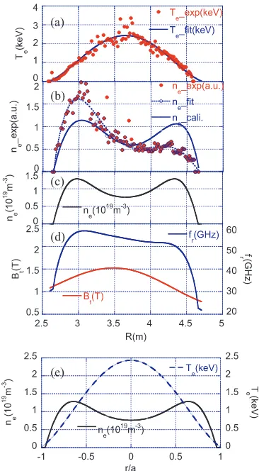
The density profile is obtained from the Thomson scattering by calibration using a microwave interferome-ter, of which the chord is equivalent to the laser beam of the Thomson scattering. The density profile is distorted due to misalignment of the laser beam. Also, the plasma center is shifted outward due to the Shafranov shift. Fig-ure 1 shows the calibration of the density profile at 1.6 s. The red closed circles indicate the experimental data. The temperature has a peaked profile, but the density profile is strongly deformed and shows a declining trend, which is caused by the misalignment of the laser beam.

To recover the density profile, we assume that the den-sity and temperature are uniform on a same magnetic sur-face. Firstly, polynomial fittings are used for the tempera-ture and density profiles,

Te fit(R)= N

n=0

anRn,

ne fit(R)= N

n=0

bnRn,

(1)

whereRis the radius, andan andbn are the fitting

coef-ficients. We useN =4 for the temperature fitting andN =8 for the density fitting. Before fitting, the data that are greatly apart from other data are removed. The plasma cen-ter (R0) is determined from the temperature profile.

Sec-ondly, we assume that thene fit(R) includes a linear trend

sincene fit(R) = ne cali(R)(1+c(R−R0)). Therefore, the

density profile can be corrected as

ne cali(R)=ne fit(R)/(c(R−R0)+1), (2)

where c is the slope of the linear fitting of the density profile. The density profile becomes quasi-symmetric (the blue solid line shown in Fig. 1(b)). Then, the density pro-file is adjusted by averaging the density ne cali(R) at the

same temperature surface. Finally, the absolute density profile (black solid line shown in Fig. 1(c)) is calibrated, as the line-integrated density equals to the microwave inter-ferometer density. Figure 1(e) shows the normalized den-sity and temperature profiles, which can be used to check the quality of the density reconstruction.

The cutoff frequency is obtained by calculating the plasma density and the toroidal magnetic field. Then the cutoffsurface can be determined. As shown in Fig. 1(d),

Fig. 1 Calibration of the reflection layer by Thomson data, (a) electron temperature profile, (b) electron density profile (before and after calibration), (c) the electron density pro-file after calibrated by microwave interferometer, (d) the toroidal magnetic field (Bt) and the X-mode cutoff fre-quency (fr). (e) The normalized density and temperature profiles. The red dots are experimental data. The large discrete peaks are removed before fitting.

the cutofflayer of 53 GHz is close to the plasma axis; how-ever, for the layers of 66 and 69 GHz, there are no cutoff layers, and the detectors receive interferential signals. We only analyze the reflection signals of 53 GHz illumination below. The plasma density is almost equal, and the cut-off layer of 53 GHz varies from 3.75 to 4.0 m (the nor-malized radius is about 0.15-0.4 m) betweent =0.9 and 2.3 s. Therefore, the curvature radius of the cutoff sur-face (≥15 cm) is larger than the illuminating beam radius (10 cm). The imaging of the fluctuation at the cutoff sur-face can be obtained using the MIR system.

3. FFT Analysis with the Ensemble

Average

signalx(t) is given by X(ω,t)=

t_+∆t

t−∆t

w(t)x(t)e−jωtdt, (3) wherew(t) is the Hanning window function, which is used to reduce the leakage of the sideband. The short-time FFT analysis is used to show the time evolution of the spectrum. In many situations, the signal from the plasma con-tains random noise. Sometimes its amplitude in the fre-quency domain is higher than the signal that we are in-terested in, and it masks the useful information. By the ensemble average technique in the frequency domain, the amplitude of the random fluctuations has an average power level in all frequency ranges. The ensemble average has less influence on the mode whose amplitude does not change in the ensemble time. Using a test parameter com-posed of a sinusoid and a random function, the qualitative effect of the noise on the signal in the frequency spectrum is shown.

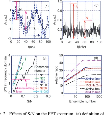
The definitions of the signal-to-noise (S/N) ratio in the time and frequency domains are illustrated in Fig. 2(a) and (b), respectively. They are defined as the amplitude ratio between the test signal and random noise. Figure 2(c) shows the ratio between the absolute amplitude of the Fourier component at the frequency of the test signal and the amplitude of the noise in the frequency domain versus the S/N ratio in the time domain. Therefore, the y-axis can be called as the S/N ratio in frequency domain. The FFT time window is set as 2 ms. Here, the black solid line denotes the ratio without average, and the others are that with different ensemble numbers. The S/N ratio in the fre-quency domain increases with the ensemble number. A larger ensemble number is suggested for lower S/N signal. Figure 2(d) shows the relative ratio between the S/N sig-nal in the frequency domain and the S/N signal in the time domain versus the ensemble number. The ratio changes greatly with the time window, but not with the signal fre-quency. The time window reflects the frequency broaden-ing. It implies that the frequency broadening affects the present S/N. The ratio decreases with the frequency width. It becomes saturated as the ensemble number increases. Therefore, the improvement by the ensemble average on the noise reduction becomes weak at a larger ensemble number. The saturated threshold of the ensemble average with a long time window is smaller than that with a short time window. If the S/N ratio is lower than 1%, it is diffi-cult to obtain the signal, even with a large ensemble num-ber.

We assume 1.5 as the discriminating level of the FFT spectrum; in other words, the FFT amplitude of the sig-nal is 1.5 times higher than the maximum amplitude of the noise in the frequency domain. By the ensemble av-erage technique, the value is about 0.03, while it is about 0.1 without the ensemble average using a 2 ms time win-dow. The distinguishable value mainly depends on the fre-quency broadening, and not on the signal frefre-quency. This

Fig. 2 Effects of S/N on the FFT spectrum. (a) definition of S/N in time domain (S/N=1 case), (b) definition of S/N in frequency domain (S/N=0.1 case), (c) the S/N in fre-quency domain versus S/N ratio in time domain, here, the y-axis is the ratio between the FFT amplitude of the test signal and the maximum amplitude of background fluctu-ation in frequency domain; (d) The relative ratio between S/N in frequency domain and S/N in time domain as a function of ensemble numbers. The signals with different frequency show similar ratio at 2 ms time window. The relative ratios with 1 ms and 4 ms time window are also plotted.

simulation only shows the qualitative effect of the noise on the signal. For the quantitative estimation, the frequency broadening should be considered. In conclusion, the en-semble technique is an effective way to reduce noise. This method requires that the lifetime of the mode be longer than the time window of the FFT. If not, the signal might be distorted by the averaging and the new analysis method that has both high-time and high-frequency ability, should be used, e.g., wavelet transforms [9, 10].

As an example of FFT analysis by the ensemble av-erage technique for analyzing the MIR signals is shown in Fig. 3, which shows the power spectrum with/without the ensemble average at 1.6 s. Here, the 4-ms time window is used for the power spectrum without the average, and 50 FFT windows with the time scale of 2 ms each are used for the power spectrum with the ensemble average. With-out the ensemble average, the MHD modes are concealed in the strong background fluctuations. The fluctuation is reduced with the ensemble average. If all the fluctuation components represent white noise, the fluctuations should be reduced to 0.14, such as the fluctuations at 60-80 kHz and 30-50 kHz. The average has less impact on the mode frequency. With the ensemble average, the fluctuation of the power is reduced significantly, and the MHD modes clearly appear.

Fig. 3 Power spectrum at 1.6 s (Top: without average and 4 ms time window is used. Bottom: with ensemble average, 50 data sections with the time scale of 2 ms each are used.)

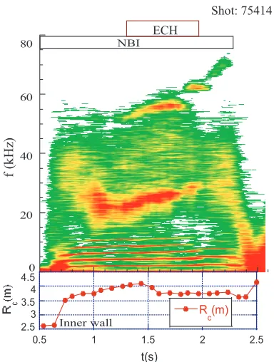
Fig. 4 Time-frequency plot of FFT spectrum, the bottom is the cutoffposition.

of the frequency spectrum and the cutoff radius. Three types of fluctuations appear in the MIR signals. In the low-frequency range, the density fluctuation has a fundamental frequency of 2.3 kHz and its higher harmonics. It appears at 0.7 s when observing the cutoffsurface, and disappears after turning offthe NBI power. The cutoffsurface varies from 3.75 to 4.0 m betweent=0.8 and 2.3 s. It seems that the onset of this mode depends on the power of the neu-tral beam, and the frequency of this mode relates to the ion temperature [11]. Att=0.9 s, a mid-frequency mode (∼23 kHz) with a wide profile appears when the plasma temperature increase to flat top. When turning on the ECH power, this frequency increases to 26 kHz, and it disap-pears after turning offthe ECH power. When turning on the ECH power, a high-frequency mode (∼55 kHz) appears. This is in the range of the Alfv´en frequency. The mode frequency increases with time, and it is up to 70 kHz at

t=2.2 s. This mode exists after turning offthe ECH power, indicating that this mode may be related to the energetic ion mode, but it is induced by the energetic electrons.

4. Cross-Correlation Analysis

The cross-power spectral analysis is used to identify the two time series that have similar spectral properties. The cross-power spectrum between the two time seriesx(t) andy(t) is defined as

Gxy(ω)=Y(ω)X(ω)∗, (4)

where the asterisk (*) denotes the complex conjugate. X(ω) andY(ω) are the discrete Fourier transforms of the time seriesx(t) andy(t), respectively. The phase shift be-tween the two time series is given by

Φxy(ω)=tan−1

⎧⎪⎪ ⎪⎨ ⎪⎪⎪⎩Im

Gxy(ω)

ReGxy(ω)

⎫⎪⎪⎪⎬_⎪⎪⎪⎭. (5)

In order to obtain the phase shift whose value corre-sponds to a high correlation in the frequency domain, the coherence spectrum is introduced, and it is defined by the cross-power spectrum normalized by the total power as

γxy(ω)= |<Gxy(ω)>|

<Gxx(ω)><Gyy(ω)>

, (6)

where the bracket (<>) denotes ensemble average. The coherency is bounded between 0 and 1, and the high value corresponds to high correlation, and zero represents com-pletely uncorrelated. The statistical confident level of the coherence spectrum is determined by the number of the in-dependent time series (1/√N).

The phase-frequency spectrum shows the dispersion relations of the MHD mode and turbulence with a distinct phase shift and propagation direction in a two-dimensional plot. It can be obtained by the two-point cross-correlation method,

S (Φ, ω)=|Gxy(ω)|δ

Φxy(ω)−Φ

. (7)

In the calculation, the delta function is replaced by a rectangular window. The width of the window depends on the number of the discrete sections in the value range of

Φxy(ω). The phase velocity and the mode number can be

obtained from the distance between two detecting points of the wave number. Substituting the phase shift for the wave number in Eq. (7), the wave number frequency spectrum [7] can be obtained.

Fig. 5 Cross-power spectrum, coherence and phase shift in the poloidal direction att=1.6 s.

been removed from every time series. When the mode ap-pears, the cross-power spectrum is peaked, and coherence becomes high. The phase shift versus frequency shows smaller jumps.

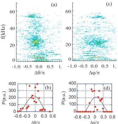
Figure 6(a) and (c) shows the contour plots of the phase-frequency spectra, log(S(Φ,ω)), in the poloidal and toroidal directions att=1.5 s, respectively. The highlight color corresponds to the large amplitude. When the mode appears, the phase shift has a peaked profile. Note that the phase shift has a broad profile, especially in the low-frequency mode. One possible reason is that the strong ef-fects of the turbulence may cause the distorted distribution of the spectrum. Another reason might be the noise. The width of the phase shift profile slightly decreases with in-creasing independent time events, and becomes constant at large time events. In this analysis, the independent events are sufficient for the ensemble average, although the life-time of the mode is not very long. Even so, the phase shift can be obtained from the fitting profile of the phase spec-trum.

The phase shift at the peak of the fitting profile is close to the ensemble phase shift <Φxy(ω)>. As shown

in Fig. 6(b), the poloidal phase shift is about 0.05πat f = 4.4 kHz. It is the same as the phase shift in Fig. 5. There-fore, the poloidal wave-number and mode number arek= 1.5 m−1 _{andm∼1, respectively. The toroidal phase shift}

is about 0.07πat f =4.4 kHz. The toroidal wave number and mode number arek=2.6 m−1_{andn∼9, respectively.}

The mode numbers of the 26 and 56 kHz arem=2/n=20, m/n=3/26, respectively. Assuming that the half width at half maximum (HWHM) of the fitting curve is the phase error, the errors of the poloidal mode numbers are about 1. The errors of the toroidal mode numbers are about 20. The phase shift has a linear trend, and the average phase velocityω/kis about 15 km/s.

The noise distorts not only the power spectrum but also the phase spectrum. When the signal is too weak, the average phase spectrum<Φxy(ω)>largely fluctuates,

as seen between 60 and 80 kHz in Fig. 5. In Fig. 6 (a) and (c), the phase shift spectrum has a broad profile. The phase

Fig. 6 (a) The phase-frequency spectrum, log(S(θ,f)), in poloidal direction at t = 1.5 s, (b) The fitting of the poloidal phase shift at f = 4.4 kHz, (c) The phase-frequency spectrum, log(S(ϕ, f)), in toroidal direction at t=1.5 s, (d) The fitting of the toroidal phase shift atf = 4.4 kHz

Fig. 7 The half width of the phase profile with different ensem-ble numbers versus S/N ratio in the phase frequency spec-trum

shift at the peak of the fitting curve is the average phase shift. The noise level of the raw signal can be estimated from the width of the phase shift. Here, the width of the phase shift profile is defined as the half width over 10% maximum in the phase shift spectrum.

square, is used in the calculation in Fig. 6. The noise level of the raw signal in estimated from the width of the phase shift. Comparing the simulation and the phase shift shown in Figs. 6(b) and (d), the S/N of MIR raw signal is about 0.05.

5. Wavelet Analysis of MIR Signals

5.1

Experiment in TPE-RX

The MIR diagnostic has been used for the density fluc-tuation measurement on the large reverse field pinch (RFP) device, TPE-RX (R =1.72 m,a =0.45 m) [14]. The 2D image of the local density fluctuation has been obtained using a 2×2 antenna array with a temporal resolution of 1µs and a spatial resolution of 3.7 cm. The probe beam with a frequency of 20 GHz in the O-mode illuminates the plasma, so that the cutoff density is 0.5 ×1019_m−3_.

The density is measured using a dual-chord interferometer. One chord passes through the plasma center and the other passes through the normalized radiusr/a=0.69. The den-sity profile is obtained by fitting the experimental data with the profile functionne(r,t) = ne(0,t)(1−r4)(1+C(t)r4).

Here, the profile factorC >1 represents the hollow den-sity, andC <1 is the peaked density profile. In this pa-per, we analyze a pulsed poloidal current drive (PPCD) plasma. In this case, the normalized cutoffradius is about 0.8-0.9 m. This region is close to the reverse field surface, and the fluctuation changes rapidly [14, 15].

5.2

Wavelet analysis

The wavelet transform of time series is its integration with the local basis functions, i.e. wavelet functions, which can be stretched and translated with flexible resolution in both time and frequency.

W(s,t)= √1 s

T+∆t

T−∆t

x(t)ψ∗

t−t s

dt, (8)

where s is the scale parameter, t is the time translation parameter, the asterisk(*) denotes the complex conjugate, and ψ(t) is the wavelet function. We use the Morlet wavelet function because it has a good balance between the time and frequency localization. Furthermore, the Morlet wavelet analysis preserves phase information that is very important for the fluctuation analysis. The Morlet wavelet waveform is a sinusoid with a Gaussian envelope, defined as

ψ(s,t)= √sexp

⎡ ⎢⎢⎢⎢⎢ ⎣iω0

t − t s

−1 2

t − t sd

2⎤

⎥⎥⎥⎥⎥ ⎦, (9)

whereω0is the dimensionless frequency,tis the

dimen-sionless time, andd is a constant related to the Gaussian envelope. Asd decreases, the time resolution improves, whereas the frequency resolution becomes worse. Asd in-creases, the Morlet wavelet reaches the Fourier transform. Here we taked=1 andω0=2π. The scale is the inverse

of the frequency, thuss=1/f [9].

The calculations of Wavelet transform can be done as a convolution, which is considerably faster in the fre-quency domain,

W(s,t)=Fˆ−1[X(ω)Ψ(ω)], (10) whereXandΨ are the Fourier transforms of the time se-riesx(t) and Morlet wavelet, respectively, and ˆF−1_{is the}

in-verse Fourier transform. Based on the same concepts in the previous section, the cross-wavelet spectrum, phase shift, and wavelet coherence can be obtained [9, 13].

5.3

Wavelet analysis of MIR data in

TPE-RX

The FFT spectrum is the integrated transform within the FFT time. It is difficult to distinguish the mode, which changes in FFT time. If we decrease the time window, the frequency resolution becomes worse. Wavelet analysis can reveal the fluctuation structure at any scale in correlation with a high-time resolution. This is advantageous to ana-lyze the fluctuation of the RFP plasma. To further under-stand the difference between the FFT and wavelet analy-sis, the toroidal cross-power spectra (shot: 52973, a PPCD plasma, cut offlayer:r/a=0.9) by FFT and wavelet trans-forms are compared in Fig. 8. Before analyzing, a band pass filter with a frequency range 5-50 kHz is used. The time window of FFT is 0.25 ms and the frequency reso-lution is 4 kHz. Therefore, it is difficult to get the mode,

Fig. 8 (a) Contour plot of the toroidal cross-power spectrum Gxy(ω,t) (FFT time window: 0.25 ms) and MIR signal

(Shot: 52973, Cut off layer: r/a =0.9), (b) Toroidal cross-wavelet spectrumWa(s,t)W_b∗(s,t). The MIR

which changes faster than 250µs. However, in the wavelet spectrum, the time duration of the structure is about 100µs. The high-frequency mode shows a shorter duration.

Fourier transform has a fixed resolution. We cannot distinguish the frequency, which changes within the FFT time. The spectrum may be transverse elongated by the in-tegration in the range of the time window. For example, the fluctuation between 30-35 kHz from 26.4 to 26.7 ms is changing both in frequency and amplitude, but it has the same frequency and amplitude in FFT. Comparing the FFT and wavelet spectra between 26.5 and 27.6 ms, the frequency evolution between 7-10 kHz in the FFT is less clear than that in the wavelet analysis. Therefore, wavelet transform can give good time resolution for high-frequency events and good frequency resolution for low-frequency events. It is sensitive to the transient fluctuation.

Since the Morlet wavelet waveform is sinusoid with Gaussian envelope, it may fail in tracking the very sharp pulses. In this case, the complex Paul wavelet function can be used [13]. On the other hand, the Morlet wavelet may fail in tracking the high-frequency components due to the low-frequency components. This problem can solved by changing the time and frequency resolutions (adjusting the parameterdin Equation (9)), or using a high-pass filter.

6. Summary

In summary, the analysis of plasma density fluctuation on LHD and TPE-RX has been performed based on MIR signals. The ensemble technique has been developed to re-duce the noise effect in the spectrum analysis. By this tech-nique, the statistical property of the fluctuation is obtained more accurately than single data. The width of the phase profile in the phase-frequency spectrum becomes wider as

the ratio of S/N in MIR raw signal is worse. MHD modes are observed during high-power NBI and ECH heating. The mode numbers are obtained by the cross-correlation technique. The wavelet analysis shows higher time and fre-quency resolutions, and the evolution of small structures is observed.

Acknowledgments

This study is supported by National Institute of Natu-ral Sciences (NIFS07KEIN0021) and by National Institute for Fusion Science (NIFS07ULPP525).

[1] S. Yamaguchiet al., Rev. Sci. Instrum.77, 10E930 (2006). [2] Y. Nagayama, S. Yamaguchi, Z.B. Shiet al, Proceedings of

ITC/ISHW2007, P1-080.

[3] R. Sabot et al., Plasma Phys. Control. Fusion. 48, B421 (2006).

[4] H. Parket al., Rev. Sci. Instrum.74, 4239 (2003). [5] E. Mazzucato, Rev. Sci. Instrum.69, 2201 (1998). [6] E.B. Hooper, Plasma Physics13, 1 (1971).

[7] Ch. P. Ritzet al., Rev. Sci. Instrum.59, 1739 (1988). [8] G.S. Xuet al., Physics of Plasmas.13, 102509 (2006). [9] A. Grinsted, J.C. Moore and S. Jevrejeva, Nonlinear

Pro-cesses in Geophysics11, 561 (2004).

[10] V.P. Budaev, I.M. Pankratov, S. Takamuraet al., Nucl. Fu-sion46, S175 (2006).

[11] S. Yamaguchi, Y. Nagayama, Z.B. Shiet al, Proceedings of ITC/ISHW2007, P1-082.

[12] T. Kass, H.S. Bosch, F. Hoenenet al., Nucl. Fusion38, 807 (1998).

[13] Christopher Torrence and Gilbert P. Compo, Bulletin of the American Meteorological Society79, 61 (1998).

[14] Y. Hinaro, Y. Maejima, T. Shimadaet al., Nucl. Fusion36, 721 (1996).