Published online November 20, 2014 (http://www.sciencepublishinggroup.com/j/acis) doi: 10.11648/j.acis.20140205.13
ISSN: 2328-5583 (Print); ISSN: 2328-5591 (Online)
A discrete-time quasi-theoretical solution of the modified
Riccati matrix algebraic equation
Tahar Latreche
Magistère in Civil Engineering, B.P. 129 Salem Lalmi, 40003 Khenchela, Algeria
Email address:
To cite this article:
Tahar Latreche. A Discrete-Time Quasi-Theoretical Solution of the Modified Riccati Matrix Algebraic Equation. Automation, Control and Intelligent Systems. Vol. 2, No. 5, 2014, pp. 87-92. doi: 10.11648/j.acis.20140205.13
Abstract:
In this paper, based on MacLaurin’s series and the Riccati equation, an algebraic quadratic equation will be developed and hence, its two roots, which represent the minimizing and maximizing optimal control matrices, would be deducted easier. Otherwise, a step-by-step algorithm to compute the control matrix for every step of time according to the preceding responses and a new signal pick will be explained. The proposed method presents a new discrete-time solution for the problem of optimal control in the linear or nonlinear cases of systems subjected to arbitrary signals. As an example, a system (structure) of three degrees of freedom, subjected to a strong earthquake is analyzed. The displacements versus time and the stiffness forces versus displacements of the system, for the two uncontrolled and controlled cases are graphically shown. Therefore, the curves of variations of the elements of the optimal control matrix versus discrete-time are also presented and clearly show the effect of the nonlinearity, of the system, which is the cause of the great responses in the uncontrolled case, and that it is optimally treated by the proposed solution. The results obtained clarify a great reduction of the controlled system results, in comparison with the uncontrolled system ones. The percentage of the differences between the controlled and uncontrolled results (displacements or stiffness forces) could even surpass 90 %, which demonstrates that the adopted solution is good even than that of the original ones of the differential or the algebraic Riccati equation.Keywords:
Optimal Control, Modified Riccati Equation, Quasi-Theoretical Solution, Discrete-Time Algorithm, Nonlinear Systems1. Introduction
It is well known that the QR is a widely used method for the optimal control of systems in engineering analysis and design practices. The method indeed, is based on the determination of the optimal control matrix, which is practically and optimally reduce the effect of the signals for which the systems are subjected. Moreover, the interest to resolve the Riccati matrix equation is appear clarify in the literature since decades, and several simple or complex algorithms are proposed [1-15 and17-23], an iterative algorithm [18], a numerical algorithm using the iterative Newton-Raphson method [1], an algorithm and a software using the Eigen-solution [6], an iterative algorithm using the iterative Newton method [8] and a step-by-step algorithm for the resolution of the differential Riccati equation [12], present some from which is published in this domain.
Otherwise, based on the matrix algebraic equation of
equation will be developed, such that its two roots which represent the closed-loop minimize and maximize optimal control matrices will be deducted easily. The deducted control matrices are computed for every so small step of time and for a given system proper matrices (deducted from the previously step of time). Therefore, the step-by-step algorithm proposed, means that the system behaves linearly during every step of time; but changing its properties from step to step in terms of the responses computed previously, so actually the proposed algorithm could be considered as a nonlinear algorithm and resolve nonlinear problems, such that the results of this method stretching well to the exact solution as-well-as the time step taken should be refined as possible.
and the acted stiffness forces on every degree of freedom show the great reductions of the results in the case of the controlled structure, compared with the others of the same uncontrolled one. Moreover, the variations of the optimal control matrix elements versus time are also shown.
Firstly, we start in the second section to transform the classical Riccati algebraic equation to a quadratic one, and therefore, we deduct in the third section, the two quasi-theoretical minimize and maximize optimal control matrices and force vector. The fourth section is appearing in the numerical example to present the results which could the proposed method offers. The following sections dealing with the explanation of results and the conclusion.
2. The Transformation of the Riccati
Equation
The state space formulation of a controlled dynamic system is stated by the ordinary differential equation
= + + (1) Where, is the controlled force vector deducted after computing the optimal control matrix, , , , are respectively, the seismic force vector, the state space response vector, and the state space matrices, given by
= − =
= − 0 − = ! 0 "
represents the unity matrix, a unity vector and the ground acceleration.
Suppose that the optimal control matrix # $%×$% (such that ' represents the number of the structure’s degrees of freedom), is related by
# = ( (2) By differentiating the Hamiltonian function we conclude the vector relations
)( = −
* ( − +
= − , *( +
= −, *( = −, *#
(3)
Expressions, such that ,%×% and +$%×$% represent the weighting matrices.
The first equation of the expressions (3) can be rewritten, after replacing ( by its expression (2), and differentiating according to
# + # = − * # − + (4)
Replacing by its relation (3) and simplifying by , we can getting then
# − # , *# + # = − * # − + (5)
Therefore, the differential matrix equation of Riccati, could be concluded as following
# = # , *# − # − * # − + (6)
Assuming that # = . # = 0, hence we could write
. # = # , *# − # − *# − + (7)
According to MacLaurin’s series, the equation (7) would be developed as follows
. # = . 0 + .,/ 0 # + .,// 0 #$⁄2 (8)
). 0 = 0 ,
*0 − 0 − *0 − + = −+
.,/ 0 = , *0 + 0 , *− + * = − + *
.,// 0 = 2 , *
(9)
Replacing . 0 , .,/ 0 and .,// 0 by their values (9), we get hence
# = , *#$ − 2 + * 3# − + (10)
The solution of the differential equation (10) couldn’t indeed extends a minimize solution, because is appearing as a mixed solution, and to separate between the minimize and maximize solutions we suppose that # = 0. Therefore, the following algebraic equation will be deducted
, *#$− + * # − + = 0 (11)
This equation represents a transformation of the matrix algebraic equation of Riccati. Therefore, the two roots of this equation represent clearly and optimally the minimizing and maximizing solutions. These roots of this equation could then be deducted easier as it is will be demonstrated in the following section for every step of time and in terms of the proper matrices of the system, computed by the step which precedes.
3. The Optimal Control Matrices and
Force Vector
The two matrix roots of the above equation (11), are given by the following expressions, which are represent the minimize and maximize optimal control matrices respectively
4# = 52 ,
*6 2 + * 3 − 72 + * 3$+ 4 , *+ 9 ⁄$
#$ = 52 , *6 2 + * 3 + 72 + * 3$+ 4 , *+ 9
$
⁄ - (12)
Otherwise, the matrix , * couldn’t have an inverse
such that it has the form , *= 70 0
Therefore, we should to proceed approximately. The proposed approximation procedure can be stated as follows
The square matrix , *+ $ could be developed by the relation
, *+ $= , * $+ 2 , * + $
Multiplying lefty the two sides of this equation by the term
, * , we get
, * , *+ $= , *+ 2 + , * $
After simplification, this equation becomes
, * 5 , *+ $− $6 = , *+ 2
The matrix 5 , *+ $− $6 has the same form as
, *, and couldn’t also have an inverse. Approximately,
we propose to take the term : instead of $, such that the coefficient : is a, as possible, stretching to the unity but not equals the strictly unity. According to the precision of the computer and/or the programming language used, we can take : precise as possible. For example we can take : =
0.9999999999999999. Then we can get approximately
, * = 5 , *+ 2 65 , *+ $− : 6 (14)
Replacing , * by its expression (14) in the two matrix roots (12), the minimize and maximize optimal control matrices which should to be computed for every step of time are then becomes
< == > ==
? # = 0.55 , *+ 2 65 , *+ $− : 6 2 + * 3 − 72 + * 3$+ 4 , *+ 9 ⁄$
# = 0.55 , *+ 2 65 , *+ $− : 6
2 + * 3 + 72 + * 3$+ 4 , *+ 9 ⁄$
- (15)
The matrix 72 + * 3$+ 4 , *+ 9 ⁄$can be computed using the iterative method [16], supposing that
A$− 72 + * 3$+ 4 , *+ 9 = 0
Such that A is the matrix square root needed.
The optimal control matrix is computed in terms the system proper matrices computed from the preceding step, such that they are in turns following the system nonlinearity laws in function of the responses computed. The optimal control forces acted to every degree of freedom of the system, for any step of time, are ranked in the vector of the third equation (3) in terms of the last step responses.
Therefore, the proposed method is summarized, for every step of time, in the following steps:
1. Computing the proper matrices of the system, according to the previously results (responses) 2. Computing, according the case, the minimize or the
maximize optimal control matrix
3. Deducting the optimal control force vector and adding it to the new exterior force vector
equation of the system to get the responses of this step of time
5. According to the results found from the step (4.), starting a new loop with a new step of time
4. Numerical Example
The chosen numerical example, for the evaluation of the efficiency of the proposed method to reduce optimally the results of the systems subjected to arbitrary signals, is imitated in a structure of three degrees of freedom with concentrates masses at the level of every degree of freedom, and subjected to the Modified El-Centro Earthquake. The stiffness behavior of the material, which the structural elements has been fabricated, is assumed to be following a bilinear model, for which it consists of two branches, an elastic branch with the stiffness equals B and a plastic branch such that the stiffness equals BC. The mass, stiffness and damping matrices for the chosen structure are given by
= DE 0 00 E 0
0 0 EF = D
B −B 0
−B B + B$ −B$
0 −B$ B$+ BGF
= H + I
E = 1 BK and B LM $ LM G can take the values: B = 25 N/E (for the elastic linear branch) and BC= B /3 (for the plastic branch), H and I represent the Rayleigh damping coefficients which are given in terms of the frequencies of the linear elastic structure Q and Q$ and the damping coefficient R. Assuming that the damping coefficient R = 0.05, then
I = 0.1 Q$− Q ⁄ Q$$− Q $ =0.006559 H = Q Q$I = 0.368488
The elastic limit displacement, with which the material stiffness transferring from the elastic to the plastic branch, is chosen to be equals 0.025 E, this limit indeed, that deciding if the proper structural stiffness and damping matrices changing or no from any step of to another. The ground acceleration variations are shown in Figure 1, such that the step of time separates two peaks is 0.02 U. The weighting matrices are chosen to be giving by
, = D0.1 00 0.1 00
0 0 0.1F + = 0
0
0 − , $ V×V
0 5 10 15 -7
-3.5 0 3.5
Time Acc
Figure 1. The acceleration of the ground (E U⁄$)
0 5 10 15
-0.5 -0.25 0 0.25
Time (s) Displacement (m)
Uncontrolled
Controlled
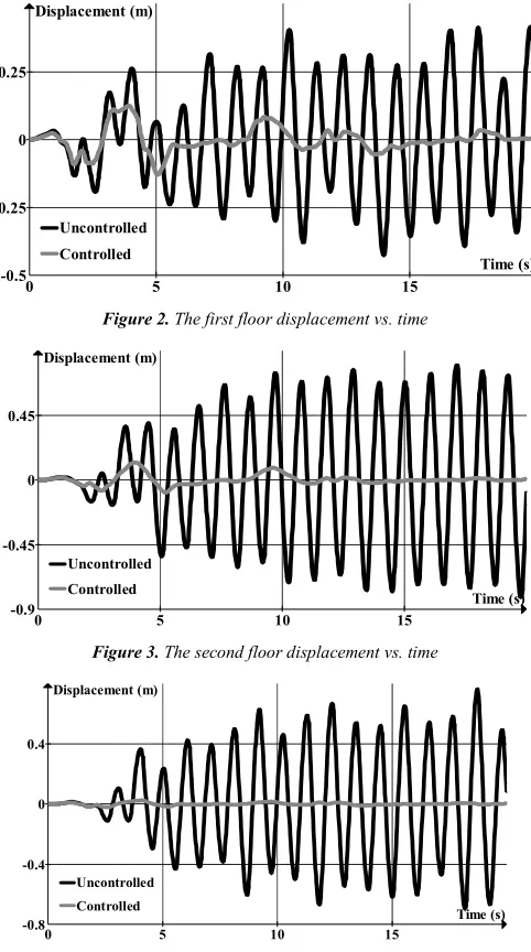
Figure 2. The first floor displacement vs. time
0 5 10 15
-0.9 -0.45 0 0.45
Time (s) Displacement (m)
Uncontrolled
Controlled
Figure 3. The second floor displacement vs. time
0 5 10 15
-0.8 -0.4 0 0.4
Time (s) Displacement (m)
Uncontrolled Controlled
Figure 4. The third floor displacement vs. time
-0.5 -0.25 0 0.25
-5 -2.5 0 2.5
Displacement (m) Force (N)
Uncontrolled Controlled
Figure 5. The first floor stiffness force vs. Displacement
-0.9 -0.45 0 0.45
-9 -4.5 0 4.5
Displacement (m) Force (N)
Uncontrolled Controlled
Figure 6. the second floor stiffness force vs. displacement
-0.8 -0.4 0 0.4
-8 -4 0 4
Displacement (m) Force (N)
Uncontrolled Controlled
Figure 7. The third floor stiffness force vs. displacement
0 5 10 15
-3 -1.5 0 1.5
Time (s) P
P66 P65 P52
0 5 10 15 -3
-1.5 0 1.5
Time (s) P
P55 P62 P45
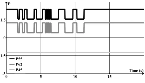
Figure 9. The P55, P62 and P45 elements of the optimal control matrix
0 5 10 15
-1.5 -0.75 0 0.75
Time (s) P
P42 P44 P41
Figure 10. The P42, P44 and P41 elements of the optimal control matrix
0 5 10 15
-0.003 -0.0015 0 0.0015
Time (s) P
P61 P64
Figure 11. The P61 and P64 elements of the optimal control matrix
5. Results and Discussion
By perceiving of the figures 2, 3 and 4 and Table1, we can remark the grand differences between the displacements of the three floors of the analyzed structure. Despite that the analyzed structure is subjected to a so strong earthquake, and the uncontrolled responses are so considerable (40 to 80 WE), we can see that the controlled responses are so moderate (3 to 13 WE) despite the fact that the elastic displacement adopted is so small too (2.5 WE), and the percentage of the differences of the three degrees of freedom displacements has being about 71 %, 85 % and 97 % from the first to the third degree of freedom respectively. The differences between the stiffness forces, for the uncontrolled and controlled cases, are also considerable, such that we can observe, by the examination of the figures 5, 6, 7 and Table 2, that the stiffness forces for the uncontrolled case are fluctuate between 4 N and 7.2 N, while these forces for the controlled case, alternate between 0.6 N and 1.5 N, and such that the
92 % for the first and the third degree of freedom.
Table 1. The maximal Uncontrolled, Controlled displacements and their fraction
Floors Uncontrolled max.
displacements
Controlled max. displacements
%
Cont./Uncont.
1 0.426 0.124 29.11
2 0.816 0.121 14.83
3 0.763 0.024 3.15
Table 2. The maximal Uncontrolled, Controlled forces and their fraction
Floors Uncontrolled max.
forces
Controlled max. forces
%
Cont./Uncont.
1 3.968 1.493 37.63
2 7.218 1.418 19.65
3 6.774 0.566 8.36
6. Conclusion
The proposed method could be summarized in determining firstly, the minimize and maximize optimal control matrices (according the case) which are the matrices roots of the quadratic equation developed herein and secondly, to compute the roots by a discrete-time algorithm which aimed to evaluate the optimal control matrix for every step of time according to the nonlinear behavior of the analyzed system which in turn (the behavior of the system), is a function of the previously responses (the displacements and velocities in the case of structural engineering). This proposed method of the optimal control of systems subjected to arbitrary signals indeed, possesses the ability to offer a good control and a so sufficiently results. Furthermore, the method allows the analysis of nonlinear systems (i.e. real systems), because it is resolved for every step of time and according to the state of the system. The figures 8-11, clearing show the effect of the nonlinearity of the structure adopted as an example, on the variations of the optimal control matrix.
The results (displacements and stiffness forces curves) of the proposed example show the efficiency of the getting solution. As it is seen by the figures and tables, the controlled results are very considerably reduced, which can surpass
90 % of percentage of the differences between uncontrolled and controlled displacements and acted stiffness forces. In spite that the ground motion acceleration are very high, and this effect is shown by the uncontrolled structure responses; but the controlled results are too moderate and sufficiency, and for the third floor, the element was not plasticized even as shown by Figure 7, despite that the limit elastic displacement adopted is very small.
References
[1] H. M. Amman, H. Neudecker, “Numerical solutions of algebraic Riccati equation”, J. of Economic Dynamics and Control, no. 21, pp. 363 - 369, 1997.
[2] B. D. O. Anderson, J. B. Moore, Linear optimal control. Prentice-Hall, 1971.
[3] B. D. O. Anderson, J. B. Moore, Optimal Filtering. Prentice-Hall, 1979.
[4] B. D. O. Anderson, J. B. Moore, Optimal control, linear quadratic methods. Prentice-Hall, 1989.
[5] Y. Arfiadi, Optimal passive and active control mechanisms for seismically excited buildings. PhD Thesis, University of Wollongong, 2000.
[6] W. F. Arnold, A. J. Laub, “Generalized eigenproblem algorithms and software for algebraic Riccati equations”, Proceedings of IEEE, vol. 72, no. 12, 1984.
[7] A. Astolfi, L. Marconi, Analysis and design of nonlinear control systems. Springer Publishers, 2008.
[8] P. Benner, J-R. Li and P. Thilo, “Numerical solution of large-scale Lyapunov equations, Riccati equations, and linear-quadratic optimal control problems”, Numerical Linear Algebra with Applications, no. 15, pp. 755 – 777, 2008.
[9] D. L. Elliott, Bilinear control systems. Springer Publishers, 2009.
[10] P. H. Geering, Optimal control with engineering applications. Springer Publishers, 2007.
[11] M. S. Grewal, A. P. Andrews, Kalman Filtering: Theory and practice. John Wiley, 2008.
[12] L. Grune, J. Pannek, Nonlinear model predictive control. Springer Publishers, 2011.
[13] A. Isidori, Nonlinear control systems 2. Springer Publishers, 1999.
[14] P. L. Kogut, G. R. Leugering, Optimal control problems for practical differential equations on reticulated domains. Springer Publishers, 2011.
[15] T. Latreche, “A discrete-time algorithm for the resolution of the Nonlinear Riccati Matrix Differential Equation for the optimal control”, American J. of Civil Engineering, no. 2, pp. 12-17, 2014.
[16] T. Latreche, “A numerical algorithm for the resolution of scalar and matrix algebraic equations using Runge-Kutta method”, Applied and Computational Mathematics, no. 3, pp. 68-74, 2014.
[17] A. Locatelli, Optimal control: an introduction. Birkhäuser Virlag, 2004.
[18] T. K. Nguyen, “Numerical solution of discrete-time algebraic Riccati equation”, Website: http://www.ictp.trieste.it/~pub-off
[19] A. Preumont, Vibration control of active structures: An Introduction. Kluwer Academic Publishers, 2002.
[20] I. L. Vér, L. L. Beranek, Noise and vibration control engineering. John Wiley, 2006.
[21] S. L. William, Control system: Fundamentals. Taylor and Francis, 2011.
[22] S. L. William, Control system: Applications. Taylor and Francis, 2011.