Numerical Method for Eulerian Vlasov Simulation Based on
Multi-Moment Scheme
∗
)
Takafumi KAWANO, Kenji IMADERA, Jiquan LI and Yasuaki KISHIMOTO
Department of Fundamental Energy Science, Graduate School of Energy Science, Kyoto University, Gokasho, Uji, Kyoto 611-0011, Japan
(Received 10 December 2010/Accepted 7 March 2011)
A new scheme referred to as the multi-moment (MM) scheme is explored to develop a more reliable Vlasov code from the viewpoint of numerical properties. The MM scheme is based on the Eulerian approach, where spatial derivatives are evaluated by interpolation functions locally constructed by not only grid values but also 0th-, 1st-, and 2nd-order moment values between grids, which largely increases numerical accuracy and resolu-tion. Through the Fourier analyses and benchmark tests of one-dimensional (1D) and 2D transport simulations, it is found that the MM scheme exhibits significantly smaller numerical dissipation and dispersion even near the Nyquist wave-number, and as a result, the MM scheme decreases the numerical cost. The MM scheme is also applied to a 1D Vlasov-Poisson simulation and we find that the scheme captures finer scale structure in veloc-ity space compared to the conservative form of interpolated differential operator (IDO-CF) scheme, while also maintaining good energy conservation.
c
2011 The Japan Society of Plasma Science and Nuclear Fusion Research
Keywords: Vlasov-Poisson simulation, conservative numerical scheme, multi-moment scheme DOI: 10.1585/pfr.6.2401097
1. Introduction
Nonlinear gyrokinetic and driftkinetic Vlasov simula-tions [1], which avoid directly solving the fast motion pro-cesses of particles with cyclotron frequencies while main-taining important kinetic effects, are considered to be an essential tool for the study of turbulent transport driven by micro-scale instabilities. Although several gyrokinetic simulations have adopted a Lagrangian (particle) approach because of limited computational resources, the Eulerian (mesh) approach is superior in reducing numerical noise and extending to an open system. Recently, with the aid of rapid progress in high-performance computing and ad-vanced numerical schemes in CFD field, the Eulerian ap-proach has become more popular in gyrokinetic simula-tions.
Several numerical schemes have been developed for solving the Vlasov equation. A splitting scheme [2] is one candidate; however, the scheme can induce a phase error associated with convection in the gyrokinetic simulation because of the nature of the semi-Lagrangian approach.
Recently, an alternative approach referred to as the conservative form of interpolated differential operator (IDO-CF) scheme [3] has been applied [4]. This scheme is based on the Eulerian approach and ensures rigorous con-servation of the integrated value over the whole system, so that the scheme can be applied to problems that require simulations over a long time scale.
author’s e-mail: [email protected]
∗)This article is based on the presentation at the 20th International Toki
Conference (ITC20).
In this paper, we explored the multi-moment (MM) scheme based on the IDO-CF one. In this scheme, spatial derivatives are evaluated by interpolation functions, which is similar in concept to the IDO-CF scheme. However, in the MM scheme, not only grid and cell-integrated (0th-order moment) values, but also 1st- and 2nd-(0th-order mo-ment values between the grids are used and time-integrated as independent variables. This feature largely improves numerical accuracy and resolution. Through the Fourier analyses [5,6] and benchmark tests of the one-dimensional (1D) and 2D transport simulations, it is found that the MM scheme exhibits significantly reduced numerical dissipa-tion and dispersion even near the Nyquist wave-number. We also applied the MM scheme to a 1D Vlasov-Poisson simulation and found that it captures finer scale structure in velocity space compared to the IDO-CF scheme.
This paper has the following outline. In Sec. 2, the nu-merical procedure of the MM scheme is briefly described. Then, we perform the Fourier analyses (in Sec. 3) and 1D (in Sec. 4) and 2D (in Sec. 5) benchmark tests to investi-gate the numerical properties of the MM scheme. The ap-plication of the MM scheme to the 1D Vlasov simulation is discussed in Sec. 6. Finally, the results are summarized with short remarks in Sec. 7.
c
2011 The Japan Society of Plasma
xj = jΔx = j Lx/Nx(j = 1,2,· · ·,Nx), where Lx and Nxare the spatial periodic length and the number of mesh
points, respectively. LetmM
j+1/2(m=0,1,2) be the value of each moment betweenxjandxj+1defined as
0M
j+1/2=
xj+1 xj
f dx/Δx, (2)
1M
j+1/2=
xj+1 xj
(x−xj)f dx/Δx2, (3)
2M
j+1/2=
xj+1 xj
(x−xj)2f dx/Δx3, (4)
wheremcorresponds to the order of the moment. Thei -th piece of -the interpolation functionFj(x) is constructed
over upwind stencils. By consideringu < 0, a left-bias interpolation can be written as
Fj(x)=a(x−xj)4+b(x−xj)3+c(x−xj)2+d(x−xj)+e. (5)
By using the five constraints for the interpolation given as
Fj(xj)= fj, Fj(xj+1)= fj+1,
xj+1 xj
Fj(x)dx/Δx=0Mj+1/2,
xj+1
xj
(x−xj)Fj(x)dx/Δx2=1Mj+1/2,
xj+1 xj
(x−xj)2Fj(x)dx/Δx3=2Mj+1/2,
(6)
the polynomial (5) is completely determined and the coef-ficients are obtained as
a=35(fj+fj+1−120Mj+1/2+601Mj+1/2
−602Mj+1/2)/Δx4,
b=−20(4fj+3fj+1−450Mj+1/2+2161Mj+1/2
−2102M
j+1/2)/Δx3,
c=30(2fj+fj+1−200Mj+1/2+901Mj+1/2
−842Mj+1/2)/Δx2,
d =−4(4fj+fj+1−300Mj+1/2+1201Mj+1/2
−1052M
j+1/2)/Δx,
e= fj.
(7)
∂t j+1/2 Δx
According to Eqs. (8-11), we can advance each value in time by using typical numerical methods such as the Runge-Kutta scheme. Note that Eq. (9) is expressed in flux form, so that0jMj+1/2becomes constant for all time-steps. As a result, the present scheme is superior in inves-tigating the problems that require simulations over a long time scale.
3. Fourier
Analysis
of
the
MM
Scheme
In this section, we present the Fourier analysis [5,6] of the MM scheme to evaluate stability and accuracy in solv-ing the 1D transport equation given by Eq. (1). When the spatial profile of a transported quantity is periodic over a domain with a uniform grid width, its grid value is decom-posed into a Fourier series
fjn= k
ˆ
fn(k) exp(ikxj), (12)
wherei = √−1 andk is the wave-number. In the MM scheme, each moment value is also decomposed as 0Mn
j+1/2=
k
0Mˆn
(k) exp(ikxj)[exp(ikΔx)−1], (13)
1Mn j+1/2=
k
1Mˆn
(k) exp(ikxj)[exp(ikΔx)−1], (14)
2Mn j+1/2=
k
2Mˆn
(k) exp(ikxj)[exp(ikΔx)−1]. (15)
In terms of Eqs. (8-11) and Eqs. (12-15), the discretized form of the time marching by the 4th-order Runge-Kutta method is written as
Fn+1=Fn+
4
p
βpAFnpΔt≡SF n,
(16)
Fn
p=F n+
4
q
αpqAFnqΔt, (17)
wheren and p denote the time-step index and the stage number of the Runge-Kutta scheme, respectively.αpq and
βp are weighted coefficients given as α21 = α32 = 1/2, α43 =1,β1 =β4 =1/6,β2 =β3 =1/3 andαpq =0 for
Fig. 1 Phase error of different schemes for the 1D linear trans-port equation. The red curve corresponds to the MM scheme, other curves correspond to the 1st-order up-wind (orange), 3rd-order upup-wind (green), IDO-CF (blue) schemes, and ideal phase (black).
Fn=
⎛ ⎜⎜⎜⎜⎜ ⎜⎜⎜⎜⎜ ⎜⎜⎜⎜⎝
ˆ
fn(k) 0Mˆ n(k)
1Mˆ n(k)
2Mˆ n
(k)
⎞ ⎟⎟⎟⎟⎟ ⎟⎟⎟⎟⎟
⎟⎟⎟⎟⎠, (18)
A=
⎛ ⎜⎜⎜⎜⎜ ⎜⎜⎜⎜⎜ ⎜⎜⎜⎜⎝
1+4C[exp(ikΔx)+4] −120C 480C −420C −C[exp(ikΔx)−1] 1 0 0
−Cexp(ikΔx) C 1 0
−Cexp(ikΔx) 0 2C 1
⎞ ⎟⎟⎟⎟⎟ ⎟⎟⎟⎟⎟ ⎟⎟⎟⎟⎠, (19)
whereC = |u|Δt/Δxdenotes the Courant number. Then, we obtain the matrix afterntime-steps as
Fn=SFn−1=S2Fn−2=· · ·=SnF0.
(20) To estimate the numerical dissipation and dispersion of each scheme, we define an amplification factor aftern
timesteps as
g(k)=|gn(k)|exp(iθn)=
ˆ
fn(k)
ˆ
f0(k), (21)
where|gn|andθnrepresent the gain and phase, respectively.
The exact solution of the gain is unity, and the exact phase isθn=CknΔx.
We examine the phase for various upwind schemes using the 4th-order Runge–Kutta time integration. Fig-ure 1 shows the phase for the 1st- and 3rd-order upwind, IDO-CF, and MM schemes. The phase is normalized as ¯
θn = θn/Cn, where the Courant number and the iteration
number are set byC =0.1 andn =1000, respectively. It is found that the MM scheme provides an accurate phase for a wide range of wave numbers in comparison with the conventional upwind schemes. Even at the Nyquist wave-number, the numerical phase error is found to be 3.1405. The normalized gain, defined as |g¯n| = |gn|1/Cn, is also
shown in Fig. 2. The gains of all schemes are less than unity for the entire region of the wave number, which en-sures numerical stability. At the Nyquist wave-number, the
Fig. 2 Gain errors of different schemes for the 1D linear trans-port equation. The correspondence of each curve is the same as in Fig. 1.
Fig. 3 Spatial accuracy of the numerical solution for the 1D transport equation by using the 1st-order upwind (or-ange), 3rd-order upwind (green), IDO-CF (blue), and MM schemes (red).
numerical gain error is found to be 0.99537. Thus, the MM scheme can achieve almost the same gain and phase as the ideal solutions, exhibiting much less dissipation and dis-persion than the other schemes.
4. Application to the 1D Transport
Simulation
To check the accuracy of the numerical solution, we applied the MM scheme incorporated with the 4th-order Runge-Kutta scheme to the 1D transport simulation, in which the governing equation is given by Eq. (1). We set the initial condition as f(t = 0,x) = 2 +sin(2πx) for 0 ≤ x ≤ 1 and the CFL number as C = 0.1. Figure 3
shows the relative numerical error σ of each upwind scheme, i.e, 1st-order upwind, 3rd-order upwind, IDO-CF, and MM scheme, whereσis defined as
σ=
Nx
j=1
|fjNume−fT ruej |
|fT ruej | . (22)
∂t +∂x[u(x,y)f(t,x,y)]
+∂
∂y[v(x,y)f(t,x,y)]=0. (23)
First, we test the case with uniform velocityu(x,y)= v(x,y)=1. The initial condition is set as
f(t=0,x,y)=2+sin(2πx) sin(2πy). (24) Figure 4 shows the relative numerical errorσof each up-wind scheme, i.e, 3rd-order upup-wind, IDO-CF and MM scheme. It can be seen that the MM scheme has a con-vergence ofΔx4.
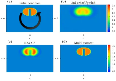
We also test the 2D solid-body rotation problem called the Zalesak problem [7]. The solid body, whose initial pro-file is shown in Fig. 5 (a), rotates with the velocity field
Fig. 4 Spatial accuracy of the numerical solution for the 2D transport equation by using the 3rd-order upwind (green), IDO-CF (blue), and MM schemes (red).
Fig. 6 Deviation from the initial values of the entropy defined
as Sn = −
i,jfin,jlnf n
i,jΔxΔv by the IDO-CF and MM schemes withNv={1024,2048}.
6. Application to the 1D
Vlasov-Poisson Simulation
Finally, we applied the MM scheme to the 1D Vlasov-Poisson simulation, which has 1D in real space and 1D in velocity space. Let us consider the normalized 1D Vlasov-Poisson equations as
∂f
∂t +v
∂f
∂x+
∂φ ∂x
∂f
∂v =0, (25)
∂2φ ∂x2 =
+∞
−∞
f dv−1, (26)
where f andφ denote the distribution function for elec-trons and the electrostatic potential, respectively; station-ary background ions are assumed. The computational do-main is defined in 0 ≤ x ≤ Lx and−vmax ≤ x ≤ vmax with a periodic boundary condition in thex-direction and is discretized by numerical grid points of (Nx,Nv−1).
Here, we investigate a benchmark test for nonlinear Landau damping with the initial condition
f(t=0,x, v)= 1 2πexp
−v2
2 1+Acos 2π
Lxx
, (27)
whereLx=4π,vmax =10,Nx=128,Δt =5×10⁻⁴, and perturbation amplitudeA=0.5. This test has been studied
in literature [4] as a fundamental test of the collisionless Landau damping and subsequent nonlinear evolution of the electrostatic field dominated by wave–particle interactions. In this study, we apply the MM scheme only in the v-direction to check the velocityspace resolution. In this case, the 0th-, 1st-, and 2nd-order moment variables corre-spond to the low-order discretized velocity moments, i.e., density, momentum and energy. They can reproduce the higher-order velocity moments balancing the transport flux in the quasi-steady state [8].
Figure 6 shows the deviation from the initial values of the entropy defined asSn = −
i,jfin,jlnf n
i,jΔxΔv by
the IDO-CF and MM schemes. It is important to con-sider the velocityspace resolution of each scheme so that the mesh number in the v-direction can be changed as
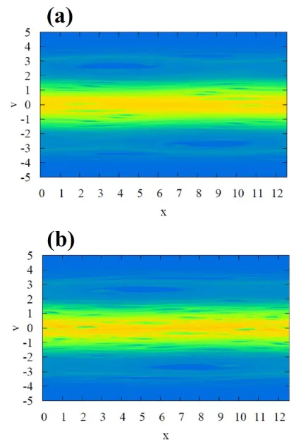
Fig. 7 Contour plots of the distribution function in phase space att = 400 by the (a) IDO-CF scheme withNv =2048
and (b) MM scheme withNv = 1024. Note that both
cases have the same memory.
Nv ={1024,2048}. It is found that the typical time scale in whichS begins to increase and also saturates is delayed by the MM scheme. Note that the IDO-CF scheme with
Nv =2048 has the same memory as the MM scheme with
Nv = 1024; however, the increase of entropy becomes faster in the former case. This demonstrates that the MM scheme captures the finer scale structure in velocity space as is also observed in the contour plots of the distribution function shown in Fig. 7.
On the other hand, the MM scheme has the same to-talenergy error level as the IDO-CF scheme. This origi-nates from the fact that the error of the totalenergy is the most sensitive toΔx, which determines the resolution of the Poisson solver. Such a tendency is similar to that ob-served in Ref. [4].