An Improved Image Denoising Using Non-Local Means Algorithm N.Gopala Krishna 1, Dr. A. Senthil Rajan2

IJSRSET1844507 | Received : 20 April 2018 | Accepted : 30 April 2018 | March-April-2018 [(4) 4 : 1490-1500]

An Improved Image Denoising Using Non-Local Means

Algorithm

N.Gopala Krishna1_{, Dr. A. Senthil Rajan}2

1_{Assoc Prof & Hod-CSE P.N.C & Viet, Repudi, Guntur , Andhra Pradesh, India}

2_{Director, Computer Center Alagappa University, Andhra Pradesh, India}

ABSTRACT

During acquistion, transmission and retrieval from storage images are corrupted with noise. In digital images the requirement for effcient image de-noising techniques has developed with the simple procedure. For researchers it is challenging task for removing noise from images. This paper presents a review of some significant work in the area of image denoising. After a brief introduction, some prevalent methodologies are characterized into various gatherings and a review of different calculations and examination is given. Bits of knowledge and potential future patterns in the territory of denoising are additionally talked about. Images denoising methods are divided into two types local and non local in local methods only exploit the spatial redundace in images. Estimation of pixel intensity based on information provided from the image and thereby utlizing the similar patters and features in images this method referred as Non local. A Non local means filter alogrithm is Non local method which estimates a noise free pixel intensity as a wegihted average of all pixel intensities in the image, and the weights are proporional to the similar between the local neighbourhood of the pixel being processed and local neighbourhoods of surrounding pixels. The method is quite spontaneous and powerul that results in comparable PSNR and visual qualit to other non-local methods.

Keywords : Image Denoising, Non-Local Means Algorithm, Digital Images, Multimedia Information Alphenomena, PSNR

I.

In all research areas digital images play an essential part in day by day life applications, for example, satellite TV, attractive reverberation imaging and technology such as geographical information systems and astronomy. Data sets collected by image sensors are generally contaminated by noise. Imperfect instruments, problems with the data acquisition process, and interfering natural phenomena can all degrade the data of interest. Furthermore, noise can be introduced by transmission errors and compression. Thus, denoising is often a necessary and the first step to be taken before the images data is analyzed. It is

necessary to apply an efficient denoising technique to compensate for such data corruption.

capacity and correspondence innovation. At the present state innovation, the main arrangement is to pack sight and sound information before its stockpiling and transmission, and decompress it at the recipient for playback. The fundamental run of pressure is to decrease the quantities of bits expected an image.

The method of image denoising is recovering the original image from noise image,

V (i) =u (i) +n (i)

They defined that this algorithm has a very fine denoising than others. It actually used a set of predetermined filters and reduced the influence of areas to denoise a pixel. But the weight is computed from the high dimensional space. The NLM (Non-local Means) method swaps every pixel by the weighted mean pixels with nearby neighborhoods. The weighting function is determined by the similarity between neighborhoods. But one of the major problems is to find the weighting function. In this research, it gives a new and unique weighting function and getting an improved NLM. This research, perform experiments to compare the weighting function against the original function, and it proves that the improved non-local algorithm outperforms the original non-local means method.

II.

Noise is the unwanted signal that affects the performance of the output signal. Noise produces undesirable effects such as unseen lines, corners, blurred objects and disturbs background scenes etc.Typical images are corrupted with additive noises modelled with both a Gaussian, uniform, or salt and pepper distribution.

Salt and Pepper Noise: Salt and pepper noise is also called as impulsive noise.Imulsive noise generate during data transmission. The image is not fully corrupted by impulsive noise, some pixel values are

changed in an image. Image pixel values are replaced by corrupted pixel values either maximum „or‟ minimum pixel value.The maximum or minimum values are dependent upon the number of bits used. In salt-and-pepper noise corresponding value for black pixels is 0 and for white pixels the corresponding value is 1. Impulsive noise can be caused by analog-todigital converter errors, bit errors in transmission, etc. The salt and pepper noise is generally caused by faulty of pixel elements in the camera sensors, faulty memory locations, or timing errors in the digitization process. Elimination of impulsive noise can be done by using dark frame subtraction and interpolating around dark/brightpixels.

Gaussian noise: Gaussian noise is also called as electronic noise because it arises in amplifiers or detectors. Gaussian noise is the statistical noise having probability density function (PDF) sequal to that of the normal distribution.This normal distribution is also known as the Gaussian distribution. This noise is additive in nature.Gaussian noise is independent at each pixel and signal intensity.It is caused by thermal noise.The mean of each pixel of an image that is affected by Gaussian noise is zero.It means that Gaussian noise qually affects each and every pixel of an image. The probability distribution function of Gaussian noise is bell shaped.

Poisson Noise: Poisson noise is also called as quantum (photon) noise or shot noise. The poisson noise is appeared due to the statistical nature of electromagnetic waves such as x-rays, visible lights and gamma rays. The x-ray and gamma ray sources emitted number of photons per unit time. These rays are injected in patient‟s body from its source, in medical x rays and gamma rays imaging systems. These sources are having random fluctuation of photons.

typically caused by statistical quantum fluctuations, that is, variation in the number of photons sensed at a given exposure level called photon shot noise. Shot noise follows a Poisson distribution, which is somehow similar to Gaussian.

Quantization noise (uniform noise) : This noise follows an approximately uniform distribution and also known as uniform noise. Quantization means the process of dividing, hence the noise caused by quantizing the pixels of a sensed image to a number of discrete levels is known as quantization noise. Though it can be signal dependent, but if dithering is explicitly applied it will be signal independent.

III.

Idan ram et.al has proposed: “Image Processing using Smooth Ordering of its Patches”. In this paper authors extracts all the patches with overlaps and order them in such a way that they are chained in the shortest possible path. The obtained ordering is applied to the corrupted image implies a permutation of the image pixels. This method enables us toobtain good recovery of clean image by applying relatively simple one dimensional smoothening operator to the recorded set of pixels.

Suhaila Sari et.al has proposed: “Development of Denoising Method for Digital Image in LowLight Condition”. In this paper authors develops a denoising method through hybridization of bilateral filters and wavelet thresholding for digital images. The major drawback of this approach was that it is not suitable to remove impulsive noise.

Lingli Huang et.al has proposed: “Improved Non-Local Means Algorithm For Image Denoising”. Image denoising technology is one of the forelands in the field of computer graphic and computer Vision. Nonlocal means method is one of the great performing methods which arouse tremendous research. In this paper, author‟s proposed an improved weighted non-local means algorithm for

image denoising. The non-local means denoising method replaces each pixel by the weighted average of pixels with the surrounding neighborhoods. The proposed method evaluates on testing images with various levels noise. Experimental results show that the algorithm improves the denoising performance. Haijuan Hu et.al has proposed “Removing Mixture of Gaussian and Impulse Noise By PatchBased Weighted Means”. Authors firstly establish a law of large numbers and a convergence theorem in distribution to show the rate of convergence of the non-local means filter for removing Gaussian noise. After that introduce the notion of degree of similarity to measure the role of similarity for the non-local means filter. Based on the convergence theorems, authors propose a patch-based weighted means filter for removing impulse noise and its mixture with Gaussian noise by combining the essential idea of the trilateral filter and that of the non-local means filter. Experiments results show that author‟s proposed filter is competitive compared to recently proposed methods.

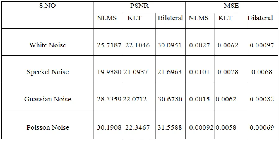
A. Jaiswal et.al. Has proposed “Image Denoising and Quality Measurements by Using Filtering and Wavelet Based Techniques”. In this paper authors have worked with denoising of salt–pepper and Gaussian noise. The work is organized in four steps as follows: (1) image is denoised by filtering method, (2) image is denoised by wavelet based techniques using thresholding, (3) hard thresholding and filtering method applied simultaneously on noisy image, (4) results of PSNR (peak signal to noise ratio) and MSE (mean square error) are calculated by comparing all cases.

and study the effect of truncation of this spectral decomposition. Second,to derive an approximation to the spectral components using the Nyström extension. Using these, authors demonstrate that this global filter can be implemented efficiently by sampling a fairly small percentage of the pixels in the image. Chandrika Saxena et.al has presented: “Noises and Image Denoising Techniques: A Brief Survey”. In this paper author reviews the existing denoising algorithms, such as filtering approach, wavelet based approach, and multifractal approach, and performs their comparative study. Different noise models including additive and multiplicative types are used. They include Gaussian noise, salt and pepper noise, speckle noise and Brownian noise. Selection of the denoising algorithm is application dependent. The filtering approach has been proved to be the best when the image is corrupted with salt and pepper noise. The wavelet based approach finds applications in denoising images corrupted with Gaussian noise.

Michael Elad et.al has presented: “Image Denoising via Sparse and Redundant Representations Over Learned Dictionaries”. Authors address the image denoising problem, where zero-mean white and homogeneous Gaussian additive noise is to be removed from a given image. The approach is based on sparse and redundant representations over trained dictionaries. Using the K-SVD algorithm, we obtain a dictionary that describes the image content effectively. Two training options are considered: using the corrupted image itself, or training on a corpus of high-quality image database. Since the K-SVD is limited in handling small image patches, we extend its deployment to arbitrary image sizes by defining a global image prior that forces sparsity over patches in every location in the image.

Florian Luisier et.al has presented: “Image Denoising in Mixed Poisson–Gaussian Noise” .Authors proposed a general methodology (PURE-LET) to design and optimize a wide class of transform-domain thresholding algorithms for denoising images

corrupted by mixed Poisson–Gaussian noise. Authors express the denoising process as a linear expansion of thresholds (LET) that optimize by relying on a purely data-adaptive unbiased estimate of the mean-squared error (MSE), derived in a non-Bayesian framework (PURE: Poisson– Gaussian unbiased risk estimate). Authors then proposed a pointwise estimator for undecimated filterbank transforms, which consists of subband-adaptive thresholding functions with signal-dependent thresholds that are globally optimized in the image domain.

Gabriela Ghimpe¸teanu et.al has presented: “A Decomposition Framework for Image Denoising Algorithms” The model computes the components of the image to be processed in a moving frame that encodes its local geometry (directions of gradients and level lines). Then, the strategy we develop is to denoise the components of the image in the moving frame in order to preserve its local geometry, which would have been more affected if processing the image directly. Experiments on a whole image database tested with several denoising methods show that this framework can provide better results than denoising the image directly, both in terms of Peak signal-to-noise ratio and Structural similarity index metrics.

IV.

1) 4.0 Non-local Means Theory

The original pixel value is lost because of noise presence in the image. To reduce the noise by using neighborhood filters like class filter which are Non local means filter by selecting each pixel I a set of pixels Si characterized by both spatial proximity and gray level values are similar the set of Si pixel values averaged by replacing the gray level value of i. The Non-Local Means (NLM) denoising algorithm uses a weighted average of pixels, within a defined search region of the image, to estimate a noise-free pixel value. The search region is usually a rectangular neighborhood, centered at the pixel of

may include pixels whose original gray value do not match the value of the original central pixel. Consequently, their participation in the averaging process degrades denoising performance. To eliminate their effect, researchers suggest creating an adaptive search-region which excludes those dissimilar pixels.

This chapter will focus on the Non-Local Means neighborhood filter that attempts to take advantage of the redundancy and self similarity of the image. The filter defines the denoised value of pixel i by applying a weighted average on the pixels assigned to the set Si. The algorithm assigns a weight to a pixel by comparing a small neighborhood around pixel j to a small neighborhood around the pixel of interest i (POI). This weight is proportional to the similarity between the pixels‟ neighborhoods. In this manner, pixels with similar neighborhood to pixel i will be assigned a higher weight, thus have a more significant contribution to the weighted average process. Consequently, NLM provides a very efficient denoising procedure that preserves edges and texture while smoothing non-textured regions.

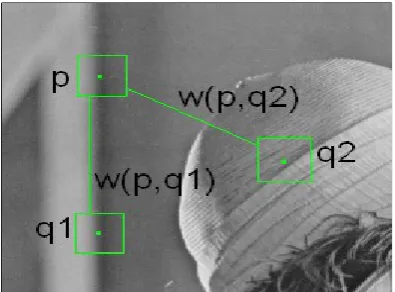
In standard NLM, all the pixels that are included in Si are used for the weighted averaging process, such that the weights are determined based on their resemblance to the POI, as explained next. Associate degree example of self-similarity is displayed in Figure one below. The figure shows 3 pixels p, q1, and q2 and their several neighborhoods. The neighborhoods of pixels p and q1 area unit similar, however the neighborhoods of pixels p and q2 don't seem to be similar. Adjacent pixels tend to possess similar neighborhoods, however non-adjacent pixels will have similar neighborhoods once there's structure within the image [1]. For instance, in Figure one most of the pixels within the same column as p can have similar neighborhoods to p's neighborhood. The self-similarity assumption will be exploited to denoise a picture. Pixels with similar neighborhoods will be accustomed confirm the denoised price of a

pixel. All pixels in that sub-set can be used for predicting the value at i. The fact that such a self-similarity exists proves image redundancy and matches the image regularity assumption.

Figure 1. In image an example of self similarity where Pixels p and q1 contains similar neighborhoods, however pixels p and q2 don't contain similar neighborhoods. Due to this, constituent q1 can have a stronger influence on the denoised worth of p over q2.

2) 4.1 Non-local Means Method

Each pixel p of the non-local means denoised image is evaluated by the following formula:

NL V p

w p , q V q

(1)

Where V is the noisy image, and weights w(p,q) meet the following conditions 0 w p , q 1 and

qw p , q 1 . Each pixel may be a weighted average of all the pixels within the video. The weights area unit supported the similarity between the neighborhoods of pixels p and alphabetic character [1, 2]. for instance, in Figure1 higher than the load w(p,q1) is way larger than w(p,q2) as a result of pixels p and q1 have similar neighborhoods and pixels p and q2 don't have similar neighborhoods. so as to reason the similarity, a locality should be outlined. Let Ni be the sq. neighborhood focused regarding pixel i with a user-defined radius Rsim. To reason the similarity between 2 neighborhoods take the weighted total of squares distinction between the 2 neighborhoods or as

a formula

d p , q

V N

V N

2

F is the neighborhood filter applied to the squared difference of the neighborhoods and will be further discussed later in this section. The weights can then be computed using the following formula:

w p , q 1

Z p e

d p , q h

Z (p) is the normalizing constant defined as

Z p

qe d p, q

h _{[1,2]. h is the weight-decay}

control parameter and will be further discussed in section 2.2.

As previously mentioned, F is the neighborhood filter with radius Rsim. The weights of F are computed by the following formula:

1

Rsim

Rsim

1 2

i

1

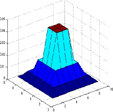
Where m is that the distance the load is from the middle of the filter. The filter provides additional weight to pixels close to the middle of the neighborhood, and fewer weights to pixels close to the sting of the neighborhood. The middle weight of F has constant weight because the pixels with a distance of 1 [3]. Despite the filter's distinctive form, the weights of filter F do total up to at least one.

Figure 2. Shape of filter F when Rsim = 4.

Equation (1) from on top of will have a special case once alphabetic character = p. this is often as a result

of the load w(p,p) are often a lot of bigger than the weights from each alternative pixel within the video. By definition this is sensible as a result of each neighborhood is analogous to itself. to stop pixel p from over-weighing itself let w(p,p) be up to the utmost weight of the opposite pixels, or in additional

mathematical terms

w p , p

max w p ,q

p q

A. Basic NL-Means algorithmic rule

The self-similarity assumptions are going to be exploited to de-noise a picture. Pixels with similar neighborhoods are going to be accustomed confirm the de-noised value of an image part. Weights unit appointed to image components on the idea of their similarity with the component being reconstructed. Whereas assessing the similarity, the video part below thought as weIl as its neighbourhood is taken into consideration. Mathematically, it'll be expressed

as [ ]( ) _{( )}∫

( | ( ) ( )| )( )

( ) ( )

The integration is carried out over all the pixels in the search window. Where

( ) ∫ ( | ( ) ( )| )( ) ( )

( ) Is a normalizing constant. is a Gaussian kerne1 and h is a filtering parameter [3]

B. Pseudo codefor NL-Means algorithm- For eachpixel x

Step1. Take a window centered in x and size (2m+1 X 2m+1), A(x,m)

Step2. Take a window centered in x and size (2n+1 X 2n+1),

W(x,n). wmax=O;

Step3. For each pixel y in A(x,m) and y different fom x,

compute the difference between W(x,n) and W(y,n) as d(x,y).

Wmax = w(x,y);

Compute the average + = w(x,y) * u(y);

Carry the sum of the weights, totalweight + = w(x, y); Step 4. Give to x the maximum of the other weights, Average + = Wmax * u(x);

Total weight + = Wmax; Compute the restored value, Rest(x) = average / totalweight;

Step 5. The distance is calculated as folIows:

Function distance (x,y,n) { distancetotal = 0 ; distance = (u (x) - u (y)r2;

For k= 1 until n {

for each i=(i1, i2) pair of integer numbers such that max ( lill, li21 ) = k

{

distance + = ( U (x + i) - u (y + i) )'2; }

aux = distance / (2*k + 1 r 2; distance total + = aux; }

Distance total / = n; }

b. The noise model

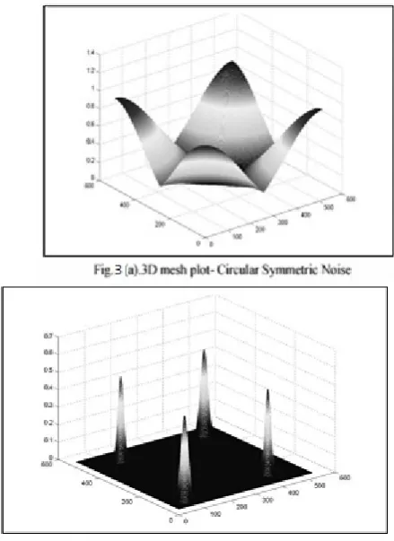
This module generates Power Spectral Density (PSD) based on [6] for completely different varieties of noise to add to the Original Clean image and get a screaky image for testing the performance of the algorithmic program. Figure l(a-b) shows 3D Mesh plot for 2 of the following noise types:

I. Adaptive White Gaussian Noise (uncorrelated) ii. Circular symmetric noise (correlated)

iii. Single line pattern noise (correlated) iv. Double line pattern noise (correlated)

Figure a pair of shows the photographs corrupted by the noise generated by the noise models. The "WelI" image could be a natural image captured by a general photographic camera, the "Barbara" and "Couple" area unit the quality information pictures.

As expressed in specific cases, single cycle of NL-Means might not evacuate the whole commotion from the video. Infinite range of neighborhoods is needed to smother the clamor completely, through an video has restricted measurements. For this case, a domestically versatile channel will keep a track of clamor distinction amid the NL-Means estimation method and later a region channel is connected in those specific ranges to uproot the remaining clamor and enhance the PSNR. This channel depends on Karhunen-Loeve remodel (KLT) that demonstrates the simplest de-corresponding ability with the unrelated coefficients and 0 mean.

4.2 Non-local Means Parameters

redundancy in any natural image by assuming that every small patch in a natural image has many similar patches in the same image. One can define a search region centered at pixel i, of size M ×M,

The non-local suggests that formula has 3 parameters. The primary parameter, h, is that the weight-decay management parameter that controls wherever the weights lay on the decaying graphical record. If h is ready too low, not enough noise are removed. If h is ready too high, the image can become muzzy. Once a picture contains racket with a customary deviation of h ought to be set between ten and fifteen. The second parameter, Rsim, is that the radius of the neighborhoods won‟t to realize the similarity between 2 pixels. If Rsim is simply too massive, no similar neighborhoods are found, however if it's too little, too several similar neighborhoods are found. Common values for Rsim square measure three and four to relinquish neighborhoods of size 7x7 and 9x9, severally [1, 2]. The third parameter, Rwin, is that the radius of a probe window. Thanks to the unskillfulness of taking the weighted average of each constituent for each constituent, it'll be reduced to a weighted average of all pixels in a very window. The window is focused at the present constituent being computed. Common values for Rwin square measure seven and nine to relinquish windows of size 15x15 and 19x19, severally [1, 2]. With this alteration the formula can take a weighted average of 152 pixels instead of a weighted average of N2 pixels for a NxN image.

V.

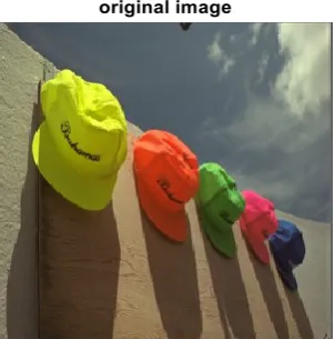
Figure 4. Above figure show original input image

Figure 5. proposed output and pervious method results

Figure 6. When applied guassian noise to input image Above shown figure X and Y are the original and the observed noisy images, respectively. It is assumed that the original image is corrupted by a Gaussian noise N with a zero mean and a known standard deviation.

Figure 7. Applied speckel noise to input image by using proposed alogrithm denoising the image and applied different pervious methods.

Figutr 8. Applied Poisson Noise to image

Tabel 1. Comparsion between Proposed Method and Pervious Methods Based On PSNR and MSE Values

VI.

A denoising method must be able to reduce as much noise as possible while preserving the original

de-noising is achieved with smoother reconstuction and less artifacts. It proves that the algorithm is spontaneous and powerfl. The proposed de-noising algorithm accomplished its goal of de-noising, improving PSNR and preserving the details, especially the edges.

Performance of denoising algorithms is measured using quantitative performance measures such as peak signal-to-noise ratio (PSNR), signal-to-noise ratio (SNR) as well as in terms of visual quality of the images. Many of the current techniques assume the noise model to be Gaussian. In reality, this assumption may not always hold true due to the varied nature and sources of noise. An ideal denoising procedure requires a priori knowledge of the noise, whereas a practical procedure may not have the required information about the variance of the noise or the noise model. Thus, most of the algorithms assume known variance of the noise and the noise model to compare the performance with different algorithms. Gaussian Noise with different variance values is added in the natural images to test the performance of the algorithm.

VII.

[1]. B. Goossens, H.Q. Luong, A.Pizuriea, W.Philips, "An Improved NonLoeal Denoising Aigorithm," lnternational Workshop on Loeal and Non-Loeal Approximation in Image Proeessing, 25-29 August 2008, Lausanne, Switzerland.

[2]. Jin Wag; Yawen Guo; Yiting Ying; Yanli Liu; QunshengPeng, "Fast Non-Loeal A1gorithm for Image Denoising", IEEE International Conferenee on lmage,Proeessing, 8- l1 Oetober 2006, Atlanta, USA.

[3]. Buades, A, ColI, B, Morel J.M, "A non-Ioeal algorithm for image denoising", IEEE Computer Soeiety Conferenee on Computer Vision andPattern Reeognition, 20-26 June 2005, San Diego, CA, USA.

[4]. Quing Xu, Hailin Jiang, Rieeardo Seopigno, Mateu Sbert, "A New Approach for Very Dark Video Denoising and Enhaneement", Proeeeding of IEEE 17th International Conferenee on Image Proeessing, 26-29 September 2010, Hongkong.Page(s):1185-1188. [5]. Jonathan Taylor, "lntroduetion to Regression

and Analysis of Varianee Robust methods", a tutorial from Depatment of Statisties, Staford University, USA.

[6]. T. Chonavel, "Statistieal Signal Proeessing- modeling and estimation", Springer lnternational Edition, 2002, lSBN 1-85233-385-5.

[7]. S.Preethi and D.Narmadha," A Survey on Image Denoising Techniques", International Journal of Computer Applications (0975 -8887) Volume 58-No.6, November 2012.

[8]. Monika Raghav, Sahil Raheja," IMAGE DENOISING TECHNIQUES:LITERATURE REVIEW", International Journal Of Engineering And Computer Science ISSN:2319- 7242.Volume 3 Issue 5 May, 2014 Page No.5637-5641.

[9]. Ajay Kumar Boyat1 and Brijendra Kumar Joshi2," A REVIEW PAPER: NOISE MODELS IN DIGITAL IMAGE PROCESSING", Signal & Image Processing : An International Journal (SIPIJ) Vol.6, No.2, April 2015.

[10]. Pooja Kaushik and Yuvraj Sharma," Comparison Of Different Image Enhancement Techniques Based Upon Psnr & Mse", International Journal of Applied Engineering Research, ISSN 0973-4562 Vol.7 No.11 (2012).

[11]. Ajay Kumar Nain et.al,"A Comparative study of mixed noise removal techniques",International Journal of Signal Processing and Pattern Recognition vol.7.No.1(2014.)