Closed Frequent Pattern Mining Using Vertical Data Format: Depth First Approach Md. Mohsin *1 , Md. Rayhan Ahmed 2, Tanveer Ahmed3

(1)

Closed Frequent Pattern Mining Using Vertical Data Format:

Depth First Approach

Md. Mohsin

*1

_{, Md. Rayhan Ahmed}

2

_{, Tanveer Ahmed}

3

1_{Department of CSE, Bangladesh University of Engineering and Technology, Dhaka, Bangladesh} 2,3_{Department of CSE, Stamford University Bangladesh, Dhaka, Bangladesh}

ABSTRACT

Frequent pattern finding plays an essential role in mining associations, correlations and many more interesting relationships among data. Discovery of such correlations among huge amount of business transaction records can help in many aspects of business-related decision-making processes like catalog design, cross-marketing and customer shopping behavior analysis. ―Market Basket Analysis‖ is one of such applications. It involves analysis of customer buying patterns by finding associations between the different items that customers place in their shopping carts. The discovery of such associations can help retailers and analysts to develop marketing strategies by gaining insight into which items are frequently purchased together by customers leading to increased sales by helping retailers do selective marketing and design efficient store layout.

Keywords: Frequent Pattern Finding, Association Rules, Vertical Data Format, Closed Frequent Itemsets.

I. INTRODUCTION

The phrase ―Frequent Pattern‖ means itemsets, subsequence or substructures that appear in a data set frequently [1]. For example, a set of items, such as tea and biscuit that appear in transaction records or customer invoices frequently and therefore it is a frequent item set. Example of a subsequence is buying first a Laptop, then a modem and then a portable speaker if it occurs frequently in a shopping database.

Another two important terms in frequent itemset mining are closed and maximal frequent pattern. An itemset is closed frequent itemset in a data set which is frequent and has no proper super-itemset having same support count. An itemset is maximal in a data set if it is frequent and there is no super itemset of which this itemset can be a subset [2]. For example, if there are two transactions: {a,b,c,d,e} and {b,c,d} and minimum support threshold is set to 1, then the set of closed frequent itemset is: C = {{a,b,c,d,e}:1}; {{b,c,d}:2} and the set of maximal frequent itemset is: M =

{{a,b,c,d,e}:1}(we cannot include {b,c,d} as maximal frequent itemset because there exists a frequent superset {a,b,c,d,e}). The set of closed frequent itemsets contains complete information of frequent itemsets. However, with the maximal frequent itemset, we can only assert two itemsets are frequent but cannot assert their actual support count.

(2)

improvement to minimize database scan and can be used in further study.

This paper concentrates on two major aspects:

 Find all frequent itemsets: By definition, each of these itemsets will occur at least as frequently as a predetermined minimum support count, min_sup.

 Generate strong association rules from frequent itemsets: By definition, these rules must satisfy minimum support (min_sup) and minimum confidence (min_conf).

Out of these two steps, the second step is much less costly then the first, so the overall performance is determined by the first step. The first step involves a major challenge of minimizing the generation of a huge number of itemsets if min_sup is set low. Because a frequent itemset guarantees each of its subsets to be frequent, so a long itemset will contain a combinatorial number of shorter, frequent sub-itemsets. For example, a frequent itemset of length 100, such as {a1, a2… a100} contains = 100 frequent 1-itemsets: a1, a2… a100, = 4950 frequent 2-itemsets: (a1, a2), (a1, a3) … (a99, a100) and so on. So total number of frequent itemsets that it contains is:

( ) ( ) ( ) ( )

This is too huge a number of itemsets for any computer to compute or store. To overcome, the concepts of closed and maximal frequent itemsets are introduced.

II. METHODS AND MATERIAL

Literature Review

In this paper we are concentrating on the three major scalable mining methods mentioned as below:

 Apriori (Agrawal & Srikant@VLDB‘94)  Frequent pattern growth (FPgrowth—Han,

Pei & Yin @SIGMOD‘00)

 Vertical data format approach (Charm— Zaki& Hsiao @SDM‘02)

Scalable mining methods are based on the Downward Closure Property of frequent patterns. That is: “Any subset of a frequent itemset must be frequent”.

For example, if the itemset {milk, bread, butter} is frequent then any subset of it like {bread, butter} or {milk, butter} is also frequent.

A. Apriori (Candidate Generation-and-Test Approach)

Apriori is the basic algorithm for finding frequent itemsets for Boolean association rules proposed by R. Agrawal and R. Srikant in 1994. It employs an iterative level-wise search and hash tree structure where k-itemsets are used to explore (k+1)-k-itemsets. They presented a property to reduce search space known as Apriori Property:

“All non-empty subsets of a frequent itemset must also be frequent”

It is based on the following observation that if an itemset I does not satisfy min_sup, then I is non-frequent. If an item A is added to the itemset I, then the resulting itemset cannot occur more frequently than I. Therefore, I∪A is not frequent either.

This property belongs to a special class of properties called anti-monotone which claims that if a set cannot pass a test, all of its supersets will fail the same test as well.

The Apriori is known as Candidate Generation and Test algorithm consisting of Join and Prune step. In the join step, the set of candidate k-itemsets Lk is generated by joining Lk-1 with itself. This joining assumes that items within a transaction or itemset are sorted in lexicographic order. In the prune step, a database scan is performed to find the candidates satisfying minimum support threshold and prune the rest. But the number of candidates can be huge therefore to reduce the size of candidates, Apriori property is applied. The subset testing to implement Apriori property can be done quickly by maintaining a hash tree of all frequent itemsets.

(3)

 Easily parallelized  Easy to implement

The disadvantages of Apriori Algorithm can be mentioned as like,

 Assumes transaction database is memory resident

 Requires many database scans  Huge number of candidates

 Tedious workload of support counting for candidates

1) Bottleneck of Frequent-pattern Mining

In Apriori, multiple database scan is incurred which is costly. Mining long patterns needs many passes of scanning and thus generates lots of candidates. To find frequent itemset i1, i2… i100.

Number of scans: 100

Number of Candidates:

( ) ( ) ( ) ( )

This is unpleasantly too huge a number of itemsets for any computer to compute or store.

2) General ideas for improving efficiency of Apriori:

a) Transaction reduction: A transaction that does not contain any frequent k-itemset is useless in subsequent scans.

b) Partitioning: Any itemset that is potentially frequent in database must be frequent in at least one of the partitions of database [4].

c) Hash-based itemset counting: A k-itemset whose corresponding hashing bucket count is below the threshold cannot be frequent [5]. d) Sampling: Mining on a subset of given data,

lower support threshold along with a method to determine the completeness.

e) Dynamic itemset counting: Add new candidate itemsets only when all of their subsets are estimated to be frequent.

f) Avoid candidate generation: Grow long patterns from short ones using local frequent items.

B. Mining Frequent Patterns using FP-Growth Approach

FP Growth is rather a different approach which mines frequent itemsets without candidate generation. It recursively grows frequent patterns by pattern and database partition. It is based on a prefix tree representation of the given database of transactions (called an FP-tree) [6], which can save considerable amounts of memory for storing the transactions. The basic idea of the FP-growth algorithm is known as Recursive Elimination Scheme inside of which a pre-processing step delete all items from the transactions that are not frequent individually and then select all transactions that contain the least frequent item and delete that item. It transforms the problem of finding long frequent patterns to search for shorter ones recursively and then concatenating the suffix. It uses the least frequent items as a suffix offering good selectivity resulting a substantially reduced search cost.

This method is capable of mining frequent patterns or frequent sequential patterns or frequent structural patterns without candidate generation which is a great improvement over Apriori algorithm.

Now it is time to discuss how FP-Growth algorithm achieved this improvement. It is actually done by using Tree Projection (described by Agarwal et al. (2001)) which:

 creates a lexicographical tree

 projects database into sub-databases based on the patterns mined so far

 recursively mines sub-databases

1) Simulation of FP-Growth Algorithm:

(4)

Figure 1. Construction ofFP-tree and Conditional Pattern Base of each item

For a large database, constructing a main-memory based FP-tree is undesirable. To overcome, first partition the database into a set of projected databases and then construct FP-tree and mine each projected database. A comparative study results that FP-Growth is efficient and scalable for mining both long and short frequent patterns and about an order of magnitude faster than Apriori algorithm and also faster than Tree-Projection algorithm.

C. Mining Frequent Pattern using Vertical Data Format

Both Apriori and FP-growth mine frequent patterns from transactional database in {TID:itemset} form known as Horizontal Data Format. Alternatively, data can be stored in the form {item:TID_set} where item is an item name and TID_set is the set of transactions containing that item and this form is known as Vertical Data Format. An algorithm known as ECLAT (Equivalence CLASS Transformation) was developed by Zaki [7] that implemented this vertical format data structure to store the transactional database.

Vertical Data Format brings a modification in the data structure by storing information in item wise fashion rather transaction-wise manner as stored in earlier algorithms. This change results only single database scan transforming into vertical format. Then it applies the Apriori property to generate (k+1)-itemsets from k-itemsets by intersecting the set of transaction IDs and unlike Apriori, this step requires no database scan because vertical data format stores complete information required for counting support.

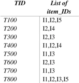
Table 1 : A Transaction Database of a Retail Shop

TID List of item_IDs

T100 I1,I2,I5

T200 I2,I4

T300 I2,I3

T400 I1,I2,I4

T500 I1,I3

T600 I2,I3

T700 I1,I3

T800 I1,I2,I3,I5

T900 I1,I2,I3

Initial step is to scan the transactional database and construct vertical data format table like as given below for the transactional database of Table-2:

Table 2: Vertical data format for transaction dataset of Table 1

itemset TID_set

I1 {T100,T400,T500,T700,T800,T900} I2 {T100,T200,T300,T400,T600,T800,T900} I3 {T300,T400,T600,T700,T800,T900} I4 {T200,T400}

I5 {T100,T800}

Now it approaches the candidate generation and test approach like Apriori and generates 2- itemsets and 3-itemsets as given below:

Table 3: Frequent 2 and 3 itemsets generation in vertical data format

Frequent 2-itemsets

itemet TID_set

I1,I2 {T100,T400,T800,

T900}

I1,I3 {T500,T700,T800,

T900}

I1,I4 {T400 }

I1,I5 {T100,T800 }

I2,I3 {T300,T600,T800,

T900}

I2,I4 {T200,T400}

I2,I5 {T100,T800}

I3,I5 {T800}

Frequent 3-itemsets

itemset TID_set

I1,I2,I3 {

T800,T90 0}

II,I2,I5 {T100,

T800}

Vertical Data Format algorithm not only takes the benefit of Apriori property to generate candidate (k+1)-itemsets from frequent k-(k+1)-itemsets, but also minimizes number of database scan to one because like Apriori it does not need to scan at each join step rather it retrieves the complete information required from vertical format table.

(5)

T700, T800, T900} and {I1, I2} = {T100, T400, T800, T900} therefore Diffset ({I1}, {I1, I2}) = {T500, T700}.

D. Comparative discussion of Scalable Algorithms

All these three algorithms have some advantages and flaws as well. Apriori uses an anti-monotone property to reduce candidate generation but involves a considerable amount of database scan which is overcome in Vertical Data format with a slight change of data structure. Moreover, FP Growth implements an approach without candidate generation but for a large database, a main memory based FP-tree is an unrealistic outcome which can be resolved by partitioning into a set of projected databases and then constructing FP-tree for each.

If the vertical data format can be added with a depth-first candidate generation out of the search space, then it can be a good variation in the evolution of mining closed frequent patterns. The point of thought is that both Vertical Data Format and Apriori algorithms employ Apriori property with a kind of breadth-first traversal of the search space which consumes a considerable memory at initial levels. If there can be implemented depth-first traversal with the vertical data format at the same time, it will result the least amount of database scan along with improved space complexity. The motivation of the paper is to develop such an algorithm which will be to some extent a blending of the benefits of the existing algorithms. Moreover, it will ultimately mine closed frequent itemsets performing additional two types of closure checking in an optimized way thus leading to the development of a closed frequent itemset mining algorithm.

III. RESULTS AND DISCUSSION

1. Proposed Algorithm

In our research work we are proposing a new algorithm named ―A Depth-first Closed Frequent Pattern & Association Rule Mining Algorithm‖. This algorithm will help to find closed frequent itemsets with an Item-wise Depth-first approach using vertical data format.

A. Input

 D, a database of transactions containing m transactions of n items;

 minsup, the minimum support count threshold  minconf, the minimum confidence threshold

B. Output

The output of the program is a full list of closed frequent itemset patterns. It will also output a list of association rules of the database of transactions containing m transactions of n items i.e. D.

C. Method

fori=1 to m do for j=1to n do

Scan database D once and store transaction’s array in

verticaldataarrayvArray fori=1 to (n-1) do

if (vArray[i].supportCount>= minsup)

while traversing tree of ith_{item in}

Depth-first manner if (any pattern with

supportCount<minsup is found or a leaf node isvisited)

Add pattern found so far longest in this branch into pattern

Backtrack;

Add nth item to patterns if vArray[an].supportCount>=minsup for each pattern S1 in patterns do for each pattern S2 in patterns do if((S1.itemCount < S2.itemCount) &&existCommonItem(S1,S2)==true)do if (S2 contains S1)

patterns.remove(S1); break;

else if (S1 is longest common subpattern of S2)

patterns.remove(S1);

for each pattern p in patterns do Store each item of p in a Set S Generate all combinations of items inS and put them in a

list L

for each combination c in L do

Take intersection of transaction_arrays of items of c

into lhs

Take intersection of

transaction_arrays of items of {S-c}intorhs

Take intersection of lhs &rhs into result

(6)

count of rhs)>=minconf) AddString.format(c.toString()+" ->"+(S-{c}).toString()) to

associationrules;

D. Simulation

Here, a simulation of the proposed algorithm on transaction database of Table-I is given below and thereby observe how the algorithm proceeds.

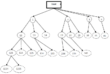
For the transaction database of Table-I with min_sup = 2, the search space traversal of the proposed algorithm is shown below:

Figure 2: Tree traversal of the proposed algorithm for the

transaction of Table-I

1) First of all, the transaction database is stored in vertical data format which is performed in Line: 1-3 of algorithm:

Table 4. Item_Id and Transaction_Array in Vertical Data Format

Item_ID Transaction Array

I1 1,0,0,1,1,0,1,1,1

I2 1,1,1,1,0,1,0,1,1

I3 0,0,1,0,1,1,1,1,1

I4 0,1,0,1,0,0,0,0,0

I5 1,0,0,0,0,0,0,1,0

2) Now the search space is traversed in Depth-First manner in Line: 4-10 of algorithm. So, first the branch 1>12>123>1234>12345 is visited. It will be found that at node ‗1234‘, min_sup constraint is not satisfied, so the longest pattern found in this branch that is ‗123‘ is added to patterns and no more node is visited in this branch.

In this manner, all the 11 nodes satisfying min_sup are added to patterns list and indicated by solid line ellipse in the tree. The dotted ellipse nodes are those patterns which are checked and pruned without branching deeper.

3) In this step, two types of closure checking: whether a pattern is a subset or a superset of another pattern and if so, remove it from patterns. This closure checking is done within line: 11-18 of the algorithm. For example, ‗123‘ is a super-node for ‗12‘, ‗23‘ and ‗13‘. To check ‗12‘ and ‗23‘ as a subset of ‗123‘, a slightly customized version of Java String function containsOf() is used. Checking of ‗13‘ to be a subset of ‗123‘ is much similar to the prominent Longest Common Subsequence problem the solution of which is also employed here. Thus, ‗1‘, ‗2‘, ‗3‘, ‗4‘, ‗12‘, ‗23‘ and ‗25‘ are removed using containsOf() function as they are subsets of ‗123‘ and ‗125‘. ‗13‘ is removed using LCS () function. Finally ‗123‘, ‗125‘ and ‗24‘ are the ultimate patterns.

4) Association rule generation for each pattern is done in this step within line: 19-27 of algorithm. For example, consider the pattern ‗123‘. First, all the combinations of ‗123‘ are derived which are: ‗1‘, ‗2‘, ‗3‘, ‘12‘, ‘13‘, ‘23‘, ‘123‘. Now for each combination, we put the combination on left hand side and the complement set on the right hand side and then calculate the ratio of support count of right side to support count of left side and if this ratio is equal or greater than the min_conf percentage, then we add this rule to associationRules as: LHS ⇒ RHS. For the pattern ‗123‘, the following rules are generated:

I1ΛI2 ⇒ I5, confidence = 2/4 = 50% I1ΛI5 ⇒ I2, confidence = 2/2 = 100% I2ΛI5 ⇒ I1, confidence = 2/2 = 100% I1 ⇒ I2ΛI5, confidence = 2/6 = 33% I2 ⇒ I1ΛI5, confidence = 2/7 = 29% I5 ⇒ I1ΛI2, confidence = 2/2 = 100%

If min_conf was set to 50%, then except 4th and 5th rules, rest will be added to the list associationRules.

2. Result Analysis

(7)

Step-1: Two nested loop scans the whole transactional database where outer loop executes m times and inner loop executes n times. So order is O(mn). If there are q no of 1s in the transactional database in total, then inside loop only q number of set operation will be executed on the vertical format data structure where 0≤q≤mn.

Step-2: Traversing the search space in depth-first manner yields a complexity of O(2a-1)p where a is the average item count in each pattern and p is the number of pattern finally obtained.

Step-3: At this step, two types of closure checking is performed on the patterns generated at previous step. A two-step nested loop is run inside of which three types of filtering is done in an if-elseif-else ladder to check whether a pattern is a superset or subset of another pattern. If S1 and S2 be two patterns containing l1 and l2 number of items respectively, then,

1. If S1 and S2 contain no common item then don‘t check further. It is O(min(l1, l2))

2. If S1 contains wholly inside S2 then remove S1. 3. If S1 is the longest common sub-pattern of S2

then remove S1. It is O(l1,l2))

So an upper bound (if case-3 is invoked for each of (2a-1)p patterns) order of Step-3 is:

where, lm=l1 = largest number of item count in a pattern

Step-4: In this step, a two level nested loop executes for each of p number of patterns generating all possible combinations of each pattern and then checking each combination whether it satisfies minimum confidence threshold.

# Outer loop executes times of number of patterns. So O(p).

# Combination generation step generates 2n-1 combinations. So O(2a-1)

# Inner loop checks min_conf constraint for each combination. So O(2a-1)

So total complexity of Step-4 is:

Total complexity of all these four steps is:

where,

m = number of transaction n = number of item

a = average item count of patterns

lm = maximum item count found in a pattern p = number of final frequent pattern

B. Experimental Setup

Programming Language: Java (JDK-1.7) IDE: NetBeans 7.1.1

Dataset: apriori.zip [8]

C. Experimental Result

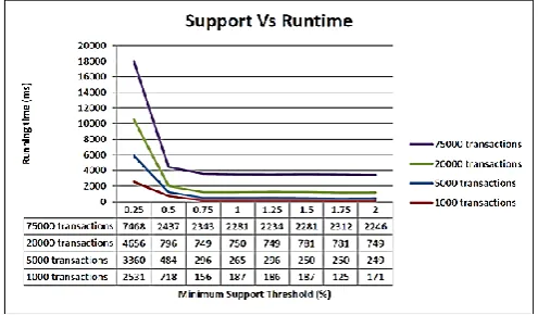
The following graph shows the running time of the proposed algorithm on a real dataset with the change of minimum support threshold and 50% confidence threshold. The code outputted the final patterns and the associated rules along with their confidence percentage:

Figure 3: Minimum support threshold Vs Runtime plot

(8)

above chart illustrates the response of the algorithm for constant confidence threshold but changed values of transaction and support threshold.

D. Comparative Analysis

1. Node Generation

In the proposed algorithm, total number of node generated after the depth-first traversal is O(2a-1)p where a is the average item count of patterns and p is the total number of patterns after refinement. It shows output-sensitivity in the node generation complexity and is equal to almost half of the generated node in Apriori in which O(n2) nodes are generated after the first join step. Moreover, at any time of the simulation, no more than 2lm nodes are stored in the stack where lm is the maximum number of item count in a pattern. So the total node generation and nodes at any level of simulation are both stable and minimized in the proposed algorithm.

2. Memory Consumption

As the Depth-First traversal is implemented, so it is obviously memory efficient and stable comparing with Apriori which implements kind of Breadth-First traversal of the search space which requires O(n2) memory at the first join step. Moreover, the data structure used for vertical data format is minimum storing each items existence in a transaction by a single bit. So comparing with Apriori, memory complexity is certainly improved.

3. Algorithm Simplicity

The proposed algorithm is much simpler than Apriori and FP-growth. The join step of Apriori is the most complex part of the algorithm which contains a long chain of if-checking. Moreover, the joining is not like the ordinary join of database operation. The FP-growth algorithm constructs a compact data structure called FP-tree which divides the whole database into several projected ones and then mine each recursively thus lacks of simplicity. On the contrary, the proposed algorithm is just traversing the search space in depth-first manner, backtracking whenever minimum support threshold is not satisfied or the leaf node found in a branch. The closure checking on these nodes is also very simple. Finally, for each pattern all combinations are generated

and then minimum confidence threshold is checked which implies the general procedure of generating association rule.

4. Running Time

The run time obtained from the simulation of the algorithm on a real large dataset containing thousands of transactions presented above implies the scalability of the algorithm. Moreover, after 0.5% of minimum support threshold, the response is almost linear shows a desired improvement with respect of candidate and associated rule generation.

IV. CONCLUSION

Frequent pattern and Association Rule mining has been a highly researched topic of Data Mining. Many researchers have been showing interest and devotion for decades in development of more efficient algorithms for mining frequent pattern in different constrained situations. Real life application of pattern mining is also a point of focus for enthusiasts. Cross-marketing decision-making and customer behavior analysis gradually becoming a matter of interest which highly recommends frequent pattern and association rule mining. Therefore, we dived into Association Rule mining as a research topic. We had done a comprehensive study of the prominent algorithms like Apriori, FP-Growth, ECLAT, CLOSET and CHARM algorithm. The comparative analysis of these algorithms led us to think of the features and drawbacks of each of these algorithms and thereby thinking of an algorithm which may perform equally or better on some real dataset. The motivation is to go through an implementation of an association rule mining algorithm and therefore observe how existing algorithms work and where improvement can be done.

(9)

number of items along with a comparative discussion based on the results obtained.

At the end, it can be concluded that association rule mining is really an interesting field of data mining to study more and more and thereby optimizing the algorithms to meet the challenge of sustaining with more difficult constraints to be provided in future.

V. REFERENCES

[1] R. Agrawal, T. Imielinski, and A. Swami. Mining association rules between sets of items in large databases. In Proc. 1993 ACM SIGMOD Int. Conf. Management of Data (SIGMOD‘93), pages 207– 216, Washington, DC, May 1993.

[2] Jiawei Han and Micheline Kamber. Data Mining: Concepts and Techniques, 2nd edition. Morgan Kaufmann, ISBN 978-1-55860-901-3

[3] R. Agrawal and R. Srikant. Fast algorithm for mining association rules in large databases. In Research Report RJ 9839, IBM Almaden Research Center, San Jose, CA, June 1994.

[4] A. Savasere, E. Omiecinski, and S. Navathe. An efficient algorithm for mining association rules in large databases. In Proc. 1995 Int. Conf. Very Large Data Bases (VLDB‘95), pages 432–443, Zurich, Switzerland, Sept. 1995.

[5] J. S. Park, M. S. Chen, and P. S. Yu. An effective hash-based algorithm for mining association rules. In Proc. 1995 ACM-SIGMOD Int. Conf. Management of Data (SIGMOD‘95), pages 175– 186, San Jose, CA, May 1995.

[6] J. Han, J. Pei, and Y. Yin. Mining frequent patterns without candidate generation. In Proc. 2000 ACM-SIGMOD Int. Conf. Management of Data (SIGMOD‘00), pages 1–12, Dallas, TX, May 2000. [7] M. J. Zaki. Scalable algorithms for association

mining. IEEE Trans. Knowledge and Data Engineering, 12:372–390, 2000.