Volatility and duration models for financial intaday data: formulation, estimation and evaluation

DOI: 10.14738/abr.66.4216.

Hassane, M. (2018). Volatility and duration models for financial intaday data: formulation, estimation and evaluation. Archives of Business Research, 6(6), 66-84.

Volatility and duration models for financial intaday data:

formulation, estimation and evaluation

Mamoudou Hassane

Lecturer, Money and International Finance,

Econometrics to the Faculty of Economics and Management of de University Abdou Moumouni of Niamey. BP 12442 Niamey – Niger.

ABSTRACT

This paper develops and tests empirically counting models for high frequency data: BIN (1,1) model with Poisson process, to check if this model allows to capture the clusturing phenomenon in the case of high frequence data, concening stocks intaday data. The process of estimation of the model using data generating process (DGP), then using the acutal data coming from three stocks of NYSE place (BOEING, DISNEY, and AWK), involves good results that validate model for generalisation to BIN(n,n) and for works on density forcasting. In this paper we studie the issue of adequacy of BIN models to capture the activities of financial markets about stocks intraday data (volume, quote, prices), and help to forecast the evolution of financial markets activities.

Key words: ACD model, count data, BIN model, clustering, density forecast. JEL classification: G14, G15.

I wish to thank Professor BAUWENS Luc, for the supervision of this work, Professor DEHEZ Pierre, Professor GIOT Pierre, all to Université Catholique de Louvain (Belgium). I am also grateful to Dr. VEREDAS David for his precious collaboration.

INTRODUCTION

It is usual to find time series consisting of count data. Such series record the number of events of a particular type occurring in a given interval. Since the data must consist of non-negative integers a model based on the normal distribution is not appropriate, although it might provide a reasonable approximation if the number of events observed in each time period is relatively large. Then for small numbers, the good distribution is a binomial process, but for a large number of observations the appropriate distribution is the Poisson. So, Poisson process should be used in the case of count data.

Considering an independent Poisson random variables, if n₁,...,n_q are independent with

) (

~ _i

i Po

n , then the total of all the counts is

) ... ( ~

... ₁

2

1 n nq Po q

n + + + + + and the counts given the total are

) ,..., , ( ~ ) ,...,

(n₁ n_q N Mult N p₁ p_q where N =n₁+...+n_q and p_i = _i ( ₁+...+ _q) i=1,...,q.

The conditional distribution is important for the analysis of log-linear models and it leads us to an analysis based on multinomial distribution.

Copyright © Society for Science and Education, United Kingdom 67 financials events as trades through autoregressive conditional duration (ACD) models, while the so-called BIN models used for count data deal with the number of events of the high frequency data (as trades) during fixed durations.

The autoregressive conditional duration (ACD) model of Engle and Russell (1998) is one of the most important models of the durations in econometric literature. It was formulated as follows:

, t t t

x = _t >0, E( _t)=1

where x_t = _{t t 1}, t=1,2,... is the length of time between financial events (trades), and the _t's are independent identical distributed (i.i.d.), with

= =

+ +

= p

j

q

j

j t j j

t j

t x

1 1

.

Here t =E

(

xt Ft 1

)

, the conditional expected waiting time. In practice Engle and Russell

(1998) have used an exponential or Weibull distribution on the { _t}. Straightforward alternative structures would be to parameterize the log _tinstead of the _t. This formulation called logACD proposed by Bauwens and Giot, allows to avoid to make constraints on parameters.

The two types of models are applied to high frequency data, particularly the financial data. The ACD models study the distribution of duration between the events (quote trades, volume or price duration), while the BIN models focus on the distribution of the number of events during a fixed length time. Then, the two types of models study the two faces of the same reality, but they could be considered as complementary than substitute.

The aim of this survey is to study the degree of relevance of BIN(1,1), the autoregressive form of the BIN models, in other words what is the degree of explanation of the financial market events, while in their paper, Rydberg and Shephard (2000) attempt to prove that, for modelling and forecasting the securities price changes on the stocks market, one could focus on N_i which are the count data.

COUNT DATA MODEL: BIN MODELS

In their paper Rydberg and Shephard (2000) proposed to model an asset price p(r) at time r

using a compound Poisson process

=

+

=

( )

1

,

)

(

)

(

r N

r t

z

o

p

r

p

₍₁₎

where {N(r)}_{r 0} is a number of trades recorded up until r and z_t is the price movement or change associated with the t-th trade. Rydberg and Shephard (2000) specified N(r) to be a counting process1_{, modelled as Cox process – that is a Poisson process with a random intensity.}

1 _{The counting process, which is used in this context, states, that if}

0

)} (

{N r _r is a process with state space

} {+

URL: http://dx.doi.org/10.14738/abr.66.4216. 68 From an economic viewpoint these authors are typically interested in comparing the rate of return on holding the asset with that obtainable by other risky investments (opportunity cost) or riskless interest rate bearing accounts. In order to do this one has to compute the return over a fixed length of time 0. Then these returns will be based around the difference

) ( } ) 1 {( +

= p i p i

p_i

+

= =

=

{( 1) }

1 ) ( 1 i N t i N t t t

z

z

+ + =

=

{ 1)

1 ) ( i N i N t t

z

.

This shows that the number of trades in the interval [i ,(i+1) ] plays a crucial role. To reflect this, Rydberg and Shephard specifies an expression as

), ( ) 1 ( +

=N i N i

Ni (2)

the number of trades in that time interval2_{. This operation called “binning operation” consists} to partitions time into sections and we count the number of trades in that interval. Notice that if N_i =0, then p_i =0, while N_i >0the prices can change. So, N_i is very important in determining the activity in the changes in the price level. For small values of there will be a negligible loss in information in doing this, compared to studying the complete record of the {

) (r

N } process.

Let the {Ni} and {zt} processes be stochastically independent and covariance stationary and

assume that the {z_t} are independent and identically distributed. Then, writing

F

_i as the information about the {N_i} sequence available infinitesimally before time i by assuming the moments exist, will be

(

p

_i

F

_i

)

=

E

{

Var

(

p

_i

N

_i

)

F

_i

}

+

Var

{

E

(

p

_i

N

_i

)

F

_i

}

Var

(

)

+

(

)

=

Var

₍

z

_t

₎

E

N

_i

F

_i

E

₍

z

_t

₎

2

Var

N

_i

F

_{i .}

Thus predicting the variance of the price over the next period of length requires modeling the mean and variance of the future number of trades. In practice E(z_t)will be too small and so what matters in the above setup is really only

E

(

N

_i

F

_i

)

.

By setting E(z_t)= 0 then

(

)

{

i s n i s i

}

{

(

i s i s

) (

i i

)

}

s i

i p ECov p p N N CovVar p N Var p N

p

Cov( 2, 2 ) 2 , 2 , ,

+ + + + + = + ). , ( ) ( 2 s i i

t Cov N N

z

Var ₊

=

Hence volatility clustering can be obtained with the autocorrelation of square price changes being proportional to the counts.

Copyright © Society for Science and Education, United Kingdom 69 A more specific result is obtained by assuming the {zt} have a first order moving average

representation ((Rydberg and Shephard (2000)). Basically empirical modeling would require the assumptions that the {N_i} and {z_t} are stochastically independent.

Poisson process Definition 1

The counting process

{

N(t),t 0

}

, is a Poisson process of rate , >0,if (i) N(0)=0

(ii) The process has independent increments, in other words the distribution is memoryless;

(iii) The number of events in any interval of length t is Poisson process with mean t. That is for all s,t 0

{

}

_{t t} n

e n s N s t N

P _{( + ) ( )= =} ( ) _{, n=0,1,...}

Note that it follows from condition (iii) that a Poisson process has stationary increments and also that

[ ]

N(t) t.

E =

which explain why is called the rate of the Poisson process.

As a prelude to giving a second definition of a Poisson process we shall define the concept of function f() being o(x).

The function f() is said to be o(x) if

0 ) ( lim

0 x =

x f

x .

Definition 2

The counting process

{

N(t),t 0

}

, is said to be a Poisson process of rate , >0, if (i) N(0)=0.

(ii) The process has stationary and independent increment. (iii)P

{

N(x)=1

}

= x+o(x)

(iv) P

{

N(x) 2

}

=o(x) .

N is a Poisson process with parameter .

[

]

i _e t

i t i t N

P = =

! ) ( )

( , t 0.

Then, under these assumptions, N(t) ~ P_O( ); the duration between events follows exponential distribution of parameter : di ~exp( ), i=1,2,... and di are independent.

The hazard function is function of , and it is constant.

The particularity of BIN models is that is random. So, this last model, will be the topic of this survey.

The model and its properties Structure of the model

URL: http://dx.doi.org/10.14738/abr.66.4216. 70 that specify the one-step ahead forecast distribution of {N_i}series using a counting distribution. In particular they specify

N

_i

F

_i ~ P_O( _i), allowing _i depending upon

F

_i

,

the information available infinitesimally before time i . Here P_O( _i), denotes a Poisson distribution with mean _i, _i is a linear function of past data as moving average models: BIN (1,1). Then the BIN(1,1) is given as follows

), (

~ _{0 i}

i

i F P

N i = + Ni 1+ i 1, (3)

which is labeled a BIN(1,1) model. Sufficient conditions for _i to be non-negative is that

. 0 ,

, This model is inspired to the GARCH model due to Bollerslev (1986) and Taylor (1986).

This model is thus autoregressive moving average (ARMA) type for

i i

i u

N = + (4)

= + N_{i 1}+ _{i 1} +u_i

i i i

i N u u

N + +

+

= ( 1 1) (5)

, )

( + ₁+ ₁

+

= N_i u_i u_i (6)

which is can be analyzed as standard multivariate ARMA models with white noise error term, where u_i =N_{i i} is such that E

(

u_i F_i

)

=0.3 _Then

i

u is conditional independent identically distributed (u_i ~ c.i.i.d ). Many of the interesting features for the BIN model follow from this structure. u_i = N_{i i} is a martingale difference (MD) which appears as an innovation for N_i. This equation (as in the case of ACD(1,1)) shows that a BIN(1,1) process corresponds to a constrained ARMA(1,1) representation for N_i, with autoregressive coefficient + , and moving average coefficient , and with a MD error term if + <1. The autocorrelation function (ACF) could be obtained by the standard formulae for the ARMA(1,1) model. Main features (mean, variance, autocorrelation function) of this model are described in following points.

Statistical properties of the BIN models

By definition, the conditional expectation of {Ni} is equal to i. Then, equation (3) allows us to

forecast expected counts, based on the information set at the previous period.

If {N_i} is generated by (3) for n with , , >0, then if + <1, the unconditional expectation ( ) and variance ( 2_{) of { }}

i

N are given by

( )

,

) (

1 +

=

=E N_i (7)

3

i

Copyright © Society for Science and Education, United Kingdom 71 2 2 2 2 2 ) ( 1 ) ( 1 2 1 + + = +

= (8)

And the autocorrelation function is derived as , ) ( 2 1 )} ( 1 { 2

1 _{+ +}

+

= ( ) 1,

1 +

= s

s s=2,3,...

Another way to compute _s is _s = _{s 1}( + ) (9)

From the expression of ( 2), it is easy to check that ( ) that measures the overdispersion, is

greater than zero. N_i becomes more dispersed than u_i when increases. From equation (8), it is easy to check that is greater than , if is greater than zero, and implies that the series observations is overdispersed.

The properties of _i are sometimes helpful, in particular E( _i)= and

= 2 ) ( _i Var 2 2 ) ( 1 + = } ) ( 1 )}{ ( 1 { 2 2 + + = .

{

( )

}

) ( ) , ( 2 i i i

i E E

N Cov = ) ( _i Var =

Generalization of BIN (1,1) model

BIN (1,1) model can be generalized as a BIN model of order p,q (BIN (p,q)) where

), (

~ O i

i i F P

N = = + + = p j q j j i j j i j i N 1 1 .

As in the standard ARMA case, p denotes the number of autoregressive terms in the model and q to denote the number of moving average ones.

We have: >0, _j >0, _j >0 that leads to the fact that _i is a non-negative sequence when

1

q with probability one. The ARMA representation of this model can be written as follows:

i i

i u

N = +

= = + + + = p j q j i j i j i j j i

jN N u u

1 1 ) ( = = + +

= max( , )

1 1 q p j q j j i j i j i

URL: http://dx.doi.org/10.14738/abr.66.4216. 72 where u_i =N_{i i} is also a martingale difference sequence and _j = _j + _j. This model is

covariance stationary when

= <

) , max(

1

. 1

q p

j j

This last assumption allows us to write the following properties

, 1 max( , )

1 =

= _pq

j j

_{( , )}= _{( )}= 2

i i

i Var N

Cov .

And Var(ui)=Var(Ni)+Var( i) 2Cov(Ni, i)

Then, one can compute easily the autocorrelation function of

{ }

N_i by using results on variances and autocorrelations of ARMA

{

max(p,q),q

}

process as in the case of BIN(1,1) form. The relevant work is focus on BIN (1,1) model.

Numerical illustrations

The first and second unconditional moments, and the autocovariances can be computed analytically as shown above. Then it is interesting to give numerical results about these moments and autocovariances for several sets of parameters.

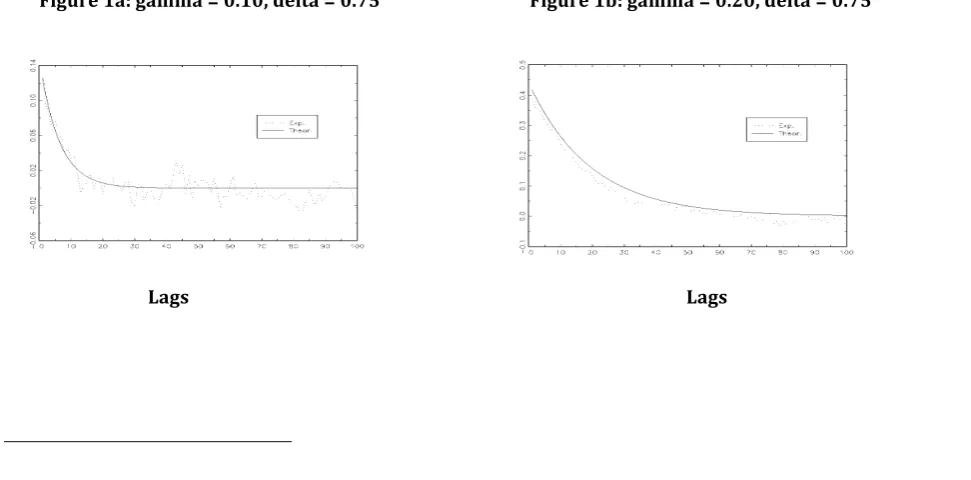
Numerical simulations allow by using (7), (8), and (9) to compute the degree of overdispersion and to get a figure (Figure 1) that plots the autocorrelation function for four set parameters4_.

Similarly as in the case for the ARCH, GARCH, and ACD class of models, close to one implies a slowly decreasing autocorrelation function, and a large value of implies a large degree of overdispersion. Figure 1 gives the graphs of the theoretical and empirical autocorrelation function.

Figure 1: Theoretical and Empirical autocorrelation functions of the BIN (1,1) model

Figure 1a: gamma = 0.10, delta = 0.75 Figure 1b: gamma = 0.20, delta = 0.75

Lags Lags

Copyright © Society for Science and Education, United Kingdom 73 Figure 1c: gamma = 0.10, delta = 0.85 Figure 1d: gamma = 0.30, delta = 0.65

Lags Lags

The figure 1c seems to exhibit the best-fitted representation of the model according to the residuals. Thus, the real values of the parameters g and d should be closed to 0.10 and 0.85 respectively. The missing parameter here is the time interval of the count data denoted D. It will be taken into account in the case of the empirical work using the actual data.

In other hand, we can examine the experimental overdispersion implied by changes in values of gamma and delta in the following table. The results are derived from a simulated data that allows a Data Generating Process.

Table 1: Overdispersion of BIN model

Coefficients Overdispersion Ratio

g = 0.10, d = .75 1.014 (1.017)

g = 0.20, d = .75 1.184 (1.187)

g = 0.10, d = .85 1.031 (1.050)

g = 0.30, d = .65 1.339 (1.386)

The overdispersion ratio is defined as the ratio of standard deviation / mean, computed according to the formula (7) and (8). We parameterize l to one, thus a = 1- g - d. In brackets we have the theoretical overdispersion ratio.

Results of Table 1 exhibit that the overdispersion ratio is an increasing function of g and decreasing function of d in BIN (1,1) model.

Estimation by Likelihood method

URL: http://dx.doi.org/10.14738/abr.66.4216. 74 density function: = otherwise N e N f _i N i i i p i i 0 ! ) ( ) ,

( for _i >0 and N_i =0,1,...

with expected value and variance _i (the rate of event occurrence, that must be greater than zero) is assumed to be an exponential linear function of a vector of explanatory variables, x_i:

) exp( )

(N_{i i} x_i

E =

A constant term as the first element of x_i is included in the program, and one can include any number of explanatory variables.

The Poisson regression model that is the standard model for count data, is a non linear regression. This regression model is hence based upon the Poisson distribution with intensity parameter that depends on covariates regressors. In the case of missing of stochastic variation, and with exact parametric dependence, with exogenous covariates, then we have the standard Poisson regression. The mixed Poisson regression is obtained if the function relating and the covariates is stochastic, likely because it involves unobserved random variables, then assumptions must be done to take into account the random term for obtaining the precise form or to come back to the standard Poisson model.

The appropriate data are cross-sectional for applied work, which consist of T independent observations, indexed by i (N_i,x_i)5_.

i

N is the number of occurrence of the event object of study, and x_i is the vector of linearly independent regressors that are thought to determine N_i

. A regression model based on this conditional distribution with a k-dimensional vector of covariates, x_i =(x_1i,...,x_ki), and parameters , through a continuous function (x_i, ), such that E

[

Ni xi

]

= (xi, ). That is to say Ni given xi is Poisson-distributed with density

(

)

! i N i i i N e x N

f = i i , Ni =0,1,2,... (1)

The log-linear form is the parameterization of the such that

) exp( _i

i = x (2)

to keep >0.

The Poisson distribution property allows us to write V

( ) ( )

n_i x_i =En_i x_i , with n_i considered as the realization of random variable N_i; then,

( )

n_i x_i exp(x_i )

E = ). exp( )... exp( )

exp(x_{1i 1} x_{2i 2} x_{ki k}

=

5 _Here

i

Copyright © Society for Science and Education, United Kingdom 75 In the likelihood-based models, the joint density of the dependent variables is specified.

By assuming that the scalar random variable N_i, given the vector of regressors x_i and parameter vector , is distributed with density f

(

N_i x_i,

)

6_{. The likelihood principle performs} as estimator of the value that maximizes the joint probability of observing the sample values

. ,...,

1 NT

N This probability is called the likelihood function, and it appears as a function of parameters conditional on the data. It is formulated as:

( )

(

)

= = T i i i x n f L 1

, , (3)

This formulation allows suppressing the dependence of L

( )

on the data and has assumed independence over i. This definition could be extended to time series data by allowing x_i to include lagged dependence and independent variables, even if it implicitly assumes cross-section data.

So, maximizing the likelihood function is equivalent to maximizing the log-likelihood function

( )

( )

(

)

= = = T i i i x n f L l 1 , ln

ln (4)

Under the so-called regularity conditions that are conditions on continuity and differentiation, the Maximum Likelihood Estimator (MLE) ˆ_ML is the solution to the first order conditions.

0 ln 1 = = = T i i f l (5)

where fi = f

(

ni xi,

)

and

l _{is a} 1

×

q vector.

The data generating process for n_i has density f

(

n_i x_i, ₀

)

where ₀ is the true parameter value. That is to say the asymptotic distribution of the MLE is usually obtained under the assumption that the density is correctly specified. Then, under the regularity conditions,

0

ˆ P _{, so the MLE is consistent for} 0.

Then,

(

)

[

1

]

0 0,

ˆ _{N A}

n d

ML , (6)

where the q× q matrix A defined as

= = T i i T f E T A 1 2 0 ln 1

lim

(7).

URL: http://dx.doi.org/10.14738/abr.66.4216. 76

Simulation

In this section, we perform an algorithm for reference sample generation then, we compute the characteristics of theoretical model (after a parameterization), and the parameters from the generate sample. We did comparison between the two generated models. We also compute the autocorrelation function (see Figure1).

By Monte Carlo simulation of discrete distribution we can perform the estimation of Poisson distribution, but there exists in Gauss the command that allows to perform the estimation of a Poisson process.

Comparison analysis

By Data Generating Process (DGP) we realize a 1,000 observations sample.

The simulation allows us, by a play on parameters to obtain the following experimental results in Table 2 below, in brackets we have the theoretical results.

Table 2: mean s.d. skewness and kurtosis of simulated data

Coefficients mean s.d. skewness kurtosis

g = 0.10, d = .75 1.021 1.035 1.050 4.153 (1.000) (1.018)

g = 0.20, d = .75 0.976 1.156 1.494 5.882 (1.000) (1.187)

g = 0.10, d = .85 1.009 1.041 1.101 4.384 (1.000) (1.050)

g = 0.30, d = .65 0.920 1.232 1.813 7.317 (1.000) (1.387)

We parameterize l to one, thus a = 1- g - d in all computations.

The results allow us to draw the following conclusion.

00 . 1

= , =0.05, =0.10, =0.85, we have the best fitted model.

Then, the means of respectively theoretical and empirical results are 1.000 and 1.009. The standard deviations of the theoretical and empirical results are respectively 1.050 and 1.041. The theoretical and empirical overdispersions are respectively 1.050 and 1.032, and are the lower overdispersion values for theoretical and empirical results. The graph of the autocorrelation function in this case indicates that it is the best-fitted model.

It is easy to check that the overdispersion coefficient, which is equal to,

N

N _{increases with .}

Another tools to check the adequacy of the model are the skewness and the kurtosis.

Copyright © Society for Science and Education, United Kingdom 77 frequency polygon) leans. Then, the skewness equal to zero implies a symmetric distribution. We can also have the case of negative or positive skewness.

The kurtosis measures a distribution’s peakedness, the degree to which one narrow range of values contains a large fraction of sample data. So, skewness indicates whether the histogram “leans to the left (negative value)” or “leans to the right (positive value)”, and kurtosis indicates how peaked it is. Their formulas are

3 2 2 3 M M

sk = , ₂

2 4

M M

kur= ,

where M_k is the kth moment of a sample of ungrouped data.

The simulation results give sk =1.10, which that the frequency curve (or density curve) leans to the right, then there are more values to the right of the model than to the left; kur=4.38 > 3, that implies a peak curve.

These results are conforming to Poisson density function.

Validation of the model: Monte Carlo method

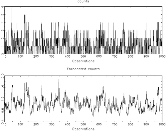
For purpose we used the data obtained by DGP for Maximum Likelihood estimation, and we get the following results in Table 3, 4, 5, 6. In brackets the fixed value of the parameter. The figures represent the graphs of counts and forecast counts.

Table 3: Estimation results by MLE using DGP count data Parameter parameter value t-stat

alpha 0.143 3.071 (0.150)

gamma 0.109 4.743 (0.100)

delta 0.752 12.981 (0.750)

Q(10) 79.87 Q(10)* 9.77

Q(10) and Q(10)* correspond respectively to the Ljung-Box Q-statistic of order 10 on counts (

i

N ) and Q-statistic on the residual u_i defined in the BIN(1,1) model. If Q is more than 18.307, then there is autocorrelation of order 10 for a threshold of 5 %.

URL: http://dx.doi.org/10.14738/abr.66.4216. 78

Figure 2: graphs of counts and forecast counts for estimation of Table 3

The results in Table 3 and the graphs of figure 2 show that the BIN(1,1) model behaves well, then the model may candidate for estimation and tests.

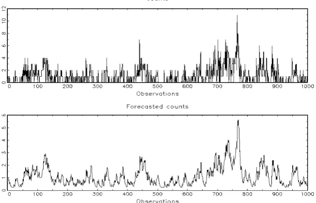
Table 4: Estimation results by MLE using DGP count data Parameter parameter value t-stat

alpha 0.068 4.546 (0.050)

gamma 0.244 9.963 (0.200)

delta 0.694 22.397 (0.750)

Copyright © Society for Science and Education, United Kingdom 79

Figure 3: graphs of counts and forecast counts for estimation of Table 4

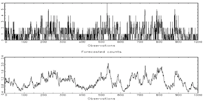
Table 5: Estimation results by MLE using DGP count data Parameter parameter value t-stat

alpha 0.038 2.464 (0.050)

gamma 0.085 5.312 (0.100)

delta 0.88 34.996 (0.850)

URL: http://dx.doi.org/10.14738/abr.66.4216. 80

Figure 4: graphs of counts and forecast counts for estimation of Table 5

It easy to check through the table 3, 4, 5 and their corresponding graphs, that the model has a good behaviour with a MLE thus, it can be used for estimation and for forecasting. There is an absence of residual autocorrelation in the three cases above. Then we can apply it for actual data.

APPLICATION TO NYSE DATA The data of three stocks

For empirical analysis, we choose a financial activity on two stocks traded on the NYSE: BOEING, DISNEY and AWK (American Water Work). The data that have been previously used for ACD by Bauwens, Giot and Veredas, were extracted from the Trade and Quote (TAQ) the database of the NYSE (for more detail, see CORE discussion paper of Bauwens and Giot (1999)). For the three stocks, we choose quote data for BOEING, quotes volume for DISNEY, and trades for AWK.

Copyright © Society for Science and Education, United Kingdom 81 counts. The count is made for a fixed length of time. In our case we use the interval of 0.25 second, 1 second and 4 seconds, and estimations are performed using each form of data. The estimation method used here is the Maximum Likelihood method. The results are analyzed through the section 3.2 below.

Estimation results

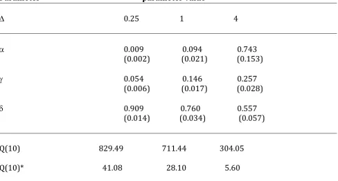
Table 6: Estimation results by MLE using quote count data for BOEING stock Parameter parameter value

D 0.25 1 4

a 0.009 0.094 0.743 (0.002) (0.021) (0.153)

g 0.054 0.146 0.257 (0.006) (0.017) (0.028)

d 0.909 0.760 0.557 (0.014) (0.034) (0.057)

Q(10) 829.49 711.44 304.05

Q(10)* 41.08 28.10 5.60

In brackets we have the standard deviation. Q(10) and Q(10)* are the Ljung-Box Q-statistic of order 10 on counts (N_i) and Q-statistic on the residual u_i defined in the BIN(1,1) model. If Q is more than 18.307, then there is autocorrelation of order 10 for a threshold of 5 %.

URL: http://dx.doi.org/10.14738/abr.66.4216. 82

Table 7: Estimation results by MLE using quote volume count data for DISNEY stock Parameter parameter value

D 0.25 1 4

a 0.002 0.020 0.548 (0.000) (0.007) (0.169)

g 0.009 0.049 0.255 (0.001) (0.008) (0.037)

d 0.984 0.931 0.608 (0.002) (0.013) (0.064)

Q(10) 375.60 332.57 523.48

Q(10)* 410.29 44.52 11.46

In brackets we have the standard deviation. Q(10) and Q(10)* are the Ljung-Box Q-statistic of order 10 on counts (N_i) and Q-statistic on the residual u_i defined in the BIN(1,1) model. D is the fixed length of time. (The number of cases is 13,795 for D = 0.25; 3,449 for D = 1; and 863 for D = 4).

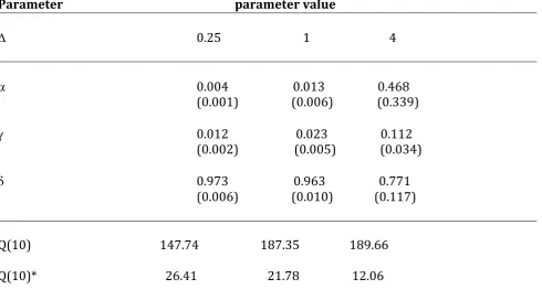
Table 8: Estimation results by MLE using trades count data for AWK stock Parameter parameter value

D 0.25 1 4

a 0.004 0.013 0.468 (0.001) (0.006) (0.339)

g 0.012 0.023 0.112 (0.002) (0.005) (0.034)

d 0.973 0.963 0.771 (0.006) (0.010) (0.117)

Q(10) 147.74 187.35 189.66

Copyright © Society for Science and Education, United Kingdom 83 In brackets we have the standard deviation. Q(10) and Q(10)* are the Ljung-Box Q-statistic of order 10 on counts (N_i) and Q-statistic on the residual u_i defined in the BIN(1,1) model. D is the fixed length of time. (The number of cases is 26,225 for D = 0.25; 6,557 for D = 1; and 1,640 for D = 4).

We can see that when the length of fixed time D increases, the values of a and g increase too. Inversely, the increases of D make d decreasing. That implies the volatility of the clustering phenomenon, and it is the basic motivation of the ARMA representation, to capture the law of the process of the high frequency counts data in financial market microstructure system.

The good results are given by the fixed length D = 4, where there is no residual autocorrelation, in the estimation of the count data of the three stocks. Then, when D increases the estimation and tests results may be better, and the volatility of the clustering is more perceptible.

CONCLUSION

The aim of this survey is to built and test BIN(1,1) model for the counts data. Before generating the data by parametrization, we used these data for estimation by the ML method for the BIN(1,1) validation. The results exhibit a good behaviour of this model, so it could be applied to the actual data. It is what we did for empirical analysis. For purpose, we use the transformed data (durations to counts), for different fixed length of time. The results of estimation of three stocks that are object of trade on the NYSE (BOEING, DISNEY, and AWK) by the Maximum Likelihood method allow to draw the following remarks. There is less dependence between the high frequency data when we consider a large value of the fixed length of time, the value of gamma becomes more and more large which increases the dispersion. The model could be generalized to take into account other variables and it could be used for density forecasting.

References

Aman, U. and David, E. A. G. (1998) “Handbook of applied economic statistics.” Marcel Dekker, inc. New York. Bauwens, L. (1999) “Recent developments in the econometrics of financial markets Using intra-day data.” CORE discussion paper 1403, Université Catholique de Louvain (UCL).

Bauwens, L. and Giot, P. (1999) “The logarithmic ACD model: an application to the bid-ask quote process of three NYSE stocks.” CORE discussion paper 9789, (UCL).

Bauwens, L. and Veredas, D. (1999) “The stochastic conditional duration model: a latent factor model for the analysis of financial duration.” CORE discussion paper 9958, UCL

Bera, A. K., and Higgins, M. L. “ARCH models: properties, estimation and testing.” Journal of Economic Survey, vol. 7, No. 4.

Colin Cameron and Pravin K. Trivedi (1998) “Regression analysis of count data.” Cambridge University Press. Dawid, P. A. (1979) “Some misleading arguments involving conditional independence.” JRSS B 41, No. 2, pp. 249-252.

Devolder, P. (1993) “Finance stochastique.” Edition de l’Université de Bruxelles.

Droesbeke, J. Fichet B. and Tassi P. (1994) “Modelisation ARCH: Theorie statistique et application dans le domaine de la Finance.” Editions de l’Université de Bruxelles, Bruxelles.

Dyckman T. and Thomas L. (1977) “Fundamental Statistics for Business and Economics.” Prentice-Hall, Inc., Englewood Cliffs, New Jersey.

Engle, R. F. (1995), “ARCH selected readings”. Oxford University Press.

Engle, R. F., and Granger, C. W. J. (1991) “Long run economic relationships: Readings in cointegration”. Oxford University Press.

URL: http://dx.doi.org/10.14738/abr.66.4216. 84 GAUSS Applications (1995) “Constrained Maximum Likelihood.” Aptech Systems, Inc. Maple Valey, USA.

Giot, P. (1999) “Time transformations, intra-day data and volatility models.” CORE discussion paper 9944, UCL. Greene, W. H. (1997), “Econometrics Analysis.” Prentice-Hall Inc. New York.

Harvey, A. C. (1990) “The Econometric Analysis of Time Series.” Second edition, Harvester Wheatsheaf. ---(1993) “Time Series Models.” Second Edition, Harvester Wheatsheaf.

Hendry, D. F. and ali (1993) “Cointegration, error correction, and the econometric analysis of non-stationary data.” Oxford University Press.

Laure, B. and Gervais, J. P. (1998) “L’Analyse des séries chronologiques: spécification et estimation des modèles univariés et multivariés.” CODESRIA, document spécial n° 9.

Lewis P. and Orav E. (1989) “Simulation methodology for Statisticians operations Analysts and Engineers.” Vol. 1 Wadsworth, Inc., Belmont, California.

Mills, T. C. (1999) “The Econometric Modeling of financial Time Series.” Second edition, Cambridge University Press.

Nerlove M., Grether D. M. and Carvalho (1979) “Analysis of Economic Time Series: A Synthesis.” Academic Press, inc. New York.

Randolph, N. (1995) “Probability, Stochastic Processes, and Queuing Theory: The Mathematics of computer performance Modeling.” Springer-Verlag New York, Inc.

Ridberg, T. and Shephard, N. (1999) “BIN models for trade-by-trade data. Modelling the number of trades in a fixed interval.” Nuffield College, Oxford, working paper series 1999-w14.

Rubinstein R. Y. (1981) “Simulation and the Monte Carlo method.” John Wiley & Sons, Inc., USA.

Sheldon M. Ross (2000) “Introduction to Probability Models.” Seventh Edition, Academic Press, San Diego, USA.

Sigles

ACD: Autoregressive Conditional Durations

ARCH: Autoregressive Conditional Heteroscedasticity ARMA: Autoregressive Moving Average

DGP: Data Generating Process GARCH: General ARCH