AN ENERGY-EFFICIENT HIERARCHICAL
CLUSTERING ALGORITHM FOR WIRELESS
SENSOR NETWORK: AN IMPROVEMENT OVER
LEACH
Mukesh Kushwaha
1, Prof. (Dr.) Bhawna Mallick
21Computer Science and Engineering, 2Dean Academics & HOD Computer Science and Engineering,
Galgotias College of Engineering and Technology, Greater Noida, (India)
ABSTRACT
A wireless network consisting of large number of small sensors with low-power transceivers. These devices rely
on battery power so that; improvement in the energy of these networks becomes important. Wireless sensor
network (WSN) require various power management protocols to reduce the power consumption. In this paper
we study that different number of clustering algorithm leads to different network performance on the energy
balancing, energy consumption and network lifetime. We propose a Multi-hop Hierarchical Stable Election
Protocol (MHSEP) for wireless sensor networks to enhance the network lifetime and avoid the formation of
energy holes. Classical clustering protocols assume that all the nodes in a system are equipped with the equal
amount of energy and as a result, network cannot take full advantage of the presence of node heterogeneity in
system. Our proposed protocol is a heterogeneous-aware protocol to increase the time-interval before the death
of first node (we refer to as stability period), which is critical for many applications where the feedback from the
sensor network must be reliable. MHSEP is a hierarchical clustering routing protocol which selects sensor
nodes with criterion of residual energy level and weighted election probabilities of each node to act as cluster
heads and establish intra-cluster multi-hop routing based on the two factors between the criteria of residual
energy level and distance. Simulation results show that our MHSEP can largely reduce the total energy
consumption and significantly increase the network lifetime compared to other routing algorithm like LEACH.
Keywords:
Clustering Method, Cluster head, Low-Energy Adaptive Clustering Hierarchy
(LEACH), MHSEP (Multi-hoping stable election protocols), Wireless Sensor Network.
I. INTRODUCTION
A Wireless Network consisting of a large number of small sensors with low-power transceivers. It can be an
effective tool for gathering data in variety of environment. Since these devices rely on battery power and may be
placed in hostile environments replacing them becomes a tedious task [1]. So that improvement in the energy of
these networks becomes important. We clustering the sensors in to group, so that sensors communicate
information only to cluster head and then cluster heads communicate the aggregate information to the
processing center this may save the energy [2].
Wireless sensor network (WSN) require various power management protocols to reduce the power consumption
generating energy-efficient protocol for wireless sensor network. This thesis describes a new protocol for energy
efficiency.
1.1 Motivation
Under classical approaches, a part of the field will not be monitored for a significant part of the lifetime of the
network, and as a result the sensing process of the field will be biased [5]. A solution proposed in , called
LEACH[6], [7] guarantees that the energy load is well distributed by dynamically created clusters, using cluster
heads dynamically elected according to a priori optimal probability. LEACH-type schemes are obtained
assuming that the nodes of the sensor network are equipped with the equal amount of energy this is the case of
homogeneous sensor network as a result, they cannot take fully utilized the presence of node heterogeneity. SEP
[8], a heterogeneous-aware protocol to increase the time-interval before the death of first node (it is stability
period), which is a crucial condition for many application where the feedback from the sensor network must be
reliable .We assume that a percentage of the node population is equipped with more energy than the remaining
nodes in the same network this is the case of heterogeneous sensor networks. In SEP there are two level of
Hierarchy and the energy distribution is not uniform practically, But it is single hop so if the node has a large
distance from destination. It consumes huge energy to transmit data, whether in Multi-hop routing the data can
be handles by others and It will consumes less energy compared to single hope. So our stability of network
improved by using multi-hop concept with heterogeneous WSN model. The energy efficiency is first priority of
our model so we propose an Energy-Efficient Multi hop Hierarchical Stable Election Protocol (MHSEP) for
wireless sensor networks to enhance the network lifetime and throughput. Simulation results show that our
MHSEP can largely reduce the total energy consumption and significantly increase the network lifetime
compared to other algorithm like LEACH. And this also improves the data loss rate of the transmission.
1.2 Our Contribution
In this paper we assume that the base-station is not energy limited (at least in comparison with the energy of
other sensor nodes) and that the coordinates of the sink and the dimensions of the area are known. We assume
that the nodes are distributed uniformly over the field and they are static. We propose a new protocol, we call
Multi hop Hierarchical Stable Election Protocol (MHSEP) for electing cluster heads in a distributed fashion in
two-level hierarchical wireless sensor networks. Unlike prior work MHSEP is heterogeneous-aware, in the sense
that election probabilities are weighted by the initial energy of a node relative to that of other nodes in the
network. MHSEP selects those nodes with the highest residual energy level and weighted election probabilities
to act as cluster heads. In each sector, we adopt a multi-hop communication protocol between normal nodes and
cluster head to reduce the cost of long distance transmission. MHSEP can make a tradeoff between the two
criteria of the distance and the residual energy during the period of the establishment of multi-hop route. We
show by simulation that MHSEP provides longer stability period and higher average throughput than current
clustering heterogeneous-oblivious protocols.
II. RELATED WORK
2.1. Conventional Energy Model
The energy model used in this paper is similar to that used by most existing energy efficient clustering
Fig.1. Radio Energy Model [9]
Many assumptions about the radio characteristics, which including dissipation of energy in transmit and receive
modes, that will change the advantages of different protocols.
In this model there is a simple model where the radio dissipates Eelec to run the transmitter or receiver circuitry
and Eamp for transmit amplifier to achieve an acceptable Eb/Na (see Fig.1.) These parameters are better than
the current state in radio design [9]. We also assume the energy loss due to channel transmission. Thus, to
transmit a massage of k-bit to a distance d using our radio model, the radio expends:
Equation (1) And for receive this message we also need the relation, the radio expends:
Equation (2)
For these ratio values, the receiving a message is not low cost operation, the protocols should not try to
minimize only the transmit distances but also number of transmit and receive operations for each of the
message. So there is assumption that the radio channel is symmetric, such that the energy required to transmit a
message from a node to other node is the same as the energy required to transmit a message from other node to
first node for a given network.
2.1.1. LEACH: Low-Energy Adaptive Clustering Hierarchy
LEACH [6], [7] is a self organizing and adaptive clustering protocol that uses randomization process to
distribute the load of energy dissipation evenly among the sensors in the network. In LEACH protocol the nodes
organize together into many local clusters, in which one node acting as the local base station (sink) or
cluster-head. In conventional clustering algorithms, it is easy to see that the sensors chosen to be cluster-heads would
die quickly and end the useful lifetime of all nodes belonging to those clusters. Thus LEACH includes
randomized rotation process of the high-energy cluster-head position such that it rotates among the various
sensors in order to not to quick die the battery of a single sensor. LEACH also performs local data fusion to
“compress” the amount of data being sent from the clusters to the sink, and reducing energy dissipation and
enhancing lifetime of system.
So to spread this energy usage over many nodes, the cluster-head nodes are not fixed; rather this position is
self-elected at different time of intervals. Let a set of C nodes might elect themselves cluster-heads at time t1, but at
time t1+t a new set C1 of nodes elect themselves as cluster-heads.
The operation of LEACH is divided into rounds, where first round started with a set-up phase, this phase the
clusters are organized by nodes, and then second phase is steady-state phase, in which data transfers to the base
station in system network. In order to minimize overhead, the steady-state phase is long compared to the set-up
phase.
2.1.2.1 Advertisement Phase
When the clusters are being created, each node has option to become a cluster-head for the current round. This
decision is based on the two factor first the percentage of cluster heads for the network (determined a priori) and
second the number of times of the node has been a cluster-head so far. This decision is made by the node by
choosing a random number between 0 and 1. If number is less than a threshold T (n) [10] then node becomes a
cluster head for this current round. The threshold is set as:
Equation (3)
Where,
n = given number of nodes.
p = the priori probability of a node being elected as a cluster-head.
r = is a current round number that is selected by a sensor node. If the random number is less than threshold value
T (n), then the respective node becomes the cluster-head.
G = the set of nodes that were not accepted as cluster head in the last “1/p” events.
Using the threshold, every node will be a cluster-head at some point within the 1/p rounds. During round 0
(r=0), each node has probability of p for becoming a cluster head in the network. The nodes that are
cluster-heads in round 0 cannot be cluster-cluster-heads for the next 1/p rounds. So that the probability of remaining nodes to
became heads must be increased. After 1/p-1 rounds, T=1 for any nodes that have not yet been
cluster-heads, and after 1/p rounds, all nodes are at least once again eligible to become cluster-heads.
2.1.2.2 Cluster Setup Phase
After advertisement phase each node has decided to which the cluster it is belongs, and it must inform the
cluster-head node that it will be a member of the cluster. Each node transmits this information massage back to
the cluster-head and again it is using a CSMA MAC protocol. During this phase also, all the cluster-head nodes
must keep their receivers on for receiving.
2.1.2.3 Schedule Creation phase
Schedule creation phase started when cluster-head node receives all the messages for nodes that would like to be
included in the cluster then scheduling will start. On the basis of number of nodes in the cluster, the cluster-head
node creates a TDMA [11], [12] protocol schedule that telling each node when it can transmit. This schedule is
broadcast back to the each node in the cluster.
2.1.2.4 Data Transmission phase
When the clusters and the TDMA schedule are created, transmission of data can begin. Assuming that nodes
have always data to send, they send data during their schedule transmission time to the cluster head. This
transmission uses a minimum amount of energy (it is chosen based on the received strength of the cluster-head
advertisement). The radio of each non cluster-head node should be turned off until the node’s allocated
transmission time, this will minimizing energy dissipation in these nodes. But the cluster-head node must keep
received, the cluster head node performs signal processing functions to compress the data into a single signal.
For example, if the data are audio or video signals, the cluster-head node can beam form the individual signals
to generate a composite signal. This composite signal is sent to the sink. Since the base station is far away, this
is a process of high-energy transmission. This is a phase of the steady-state operation of LEACH networks.
After a certain time of period, which is determined by a priori, the next round begins with each node
determining if it should be a cluster-head for this round and advertising this information, as described above[5],
[6].
2.2 Heterogeneous Wsn Model
Heterogeneous model describe our model of a wireless sensor network with unequal energy distribution of node
initially. We present the setting, the energy model, and how the optimal number of clusters can be computed.
We assume the case that a percentage of sensor nodes are keeping with more energy resources than the rest of
the nodes. Assuming m is the fraction (part) of the total number of nodes say n, which are equipped with α
(alpha) times more energy than the others nodes [8]. We refer to these nodes as advanced nodes because they
have more energy, and the remaining (1 − m) × n are normal nodes. We assume that all nodes are in distributed
uniformly over the sensor field.
2.2.1 SEP: Stable Election Protocol
LEACH so that in the homogeneous case the unstable region can be short. After the death of the first node, all
remaining nodes are dying on average rate within a small number of rounds as the consequence of the uniformly
remaining energy due to well distributed energy consumption. When the system is operates in the unstable
region, if the spatial density of the sensor network is large, there is a probability that a large number of nodes be
elected as cluster heads for a significant part of the unstable region (as long as the population of the nodes has
not decreased significantly). In this case, even though the system is unstable in this region, we have a relatively
reliable clustering process. The same can be noticed even if the spatial density is low but the probability is large.
SEP protocol will improves the stable region of the clustering hierarchy algorithm using the parameters of
heterogeneity, the fraction of advanced nodes (m) and the additional energy factor between advanced nodes and
normal nodes (α).
To increase the stable region, SEP attempts to maintain the condition criteria of well balanced energy
consumption. It is more possibility that advanced nodes have to become cluster-heads more often than the
normal nodes having less energy; this is equivalent to a fairness constraint on energy consumption. But that the
new heterogeneous setting (with advanced and normal nodes) has no effect on the spatial density of the network
so the a priori setting of popt, from Equation (3) describe above, does not change. On the other hand, the total
energy of system changes. Let assume that Eo is the initial energy of each normal sensor. The energy of each
advanced node will be Eo· (1 + α). The total energy of the new heterogeneous setting is equal to:
Equation (4)
So, the total energy of the system is increased by (1+α ·m) times. There is an improvement to the existing
LEACH is to increase the probability of sensor network in proportion to the energy increment.
To optimize the stable region of the system, the new method epoch must become equal to 1/popt · (1 + α · m)
because the system has α · m times more energy and virtually α · m more nodes (with the same energy as the
normal nodes).
(i) Each normal node becomes a cluster head once every 1/popt· (1+α ·m) rounds per epoch.
(ii) Each advanced node becomes a cluster head exactly 1+α times every 1/popt· (1+α·m) Rounds per epoch.
(iii) The average number of cluster heads per round per epoch is equal to n × popt (the spatial density does not
change).
2.3 Network Model
In this model we assume that all the sensor nodes are deployed in a circular area with a radius of R, and there is
no big obstacle between source node and sink node. All the sensor nodes are homogeneous and stationary. The
sensor node is location-aware and each sensor node has the capability of transmitting data to the sink node
directly. The entire network only has one sink node and it is located at the center of the area. Source nodes can
adjust their transmission power according to the relative distance to target nodes. We assume the optimal cluster
number k is 5, and then divide the circle network with radius R into 5 equal sectors. N sensors are
approximating evenly distributed in each sector and continuously monitor their surrounding environment.
We use the similar energy model as that of LEACH [6[, [7], [9]. Based on the distance between the source and
target nodes, a free space or multi-path fading channel models are used.
2.3.1 MHRP: Energy-Efficient Multi-hop Hierarchical Routing Protocol
Network performance can be significantly improved by using proper hierarchical routing protocol. Based on the
network topology, we can simply classify the routing protocols as flat routing protocols and hierarchical routing
protocols. In flat routing protocols, sensor nodes are on the equal terms. Data is routed from sensor nodes to the
sink node using routing protocols such as Direct diffusion and Rumor [13] etc. Compared with the flat routing
protocols, hierarchical routing protocols often divide the sensor nodes into cluster heads and normal nodes. The
entire network is composed of clusters consisting of cluster heads and several normal nodes. Cluster heads can
process, filter and aggregate data sent by ordinary cluster members among clustering algorithms. They are in
charge of coordinating the work of the cluster members and forwarding the processed data. However, cluster
heads rotation will generate additional energy overhead and consume major energy in aggregating and
transmitting data. So an energy-efficient mechanism for cluster heads election and rotation is necessary and
particularly important.
MHRP [14] prefer to select sensor nodes with the highest energy level to act as cluster heads and establish
routing path based on the residual energy and distance between sensor nodes. Based on the energy model of, we
argue that different cluster number has different influence on network performance, such as the energy
consumption, and the network lifetime, and get the optimal cluster number to minimize the energy consumption.
On the basis, we divide the sensor network area into several regions where we choose nodes with the highest
residual energy level as cluster heads and adopt multi-hop manner to transmit data. MHRP can ensure relatively
uniform distribution of cluster heads in entire network and save energy which contributes to prolong the
network lifetime.
2.3.1.1. Cluster Formation
Cluster formation is performed as a distributed algorithm at the beginning of data collection. Each sector has
only one cluster head that manages the data collected from the normal nodes and relays the aggregated data to
the sink node. To balance the energy consumption levels, we use the initial energy level to select the cluster
head candidates.
Due to the inflection of data volume and node location, some sensor nodes may consume large amount of
energy through long-distance transmission. For that reason, we set a multi-hop routing protocol for intra-cluster
routing. For any cluster member nodes Si, the energy consumption [6] it will cost to send data directly to its
cluster head CHsi is represented by equation 1and 2.Where k is size of bit massage and d is the distance between
Si and CHsi.
In the same environment, suppose a node Si chooses another node Sj which can communicate with the cluster
head CHsi directly as its relay node. We adopt a free space propagation channel model to deliver a k-bits packet
to cluster heads. The energy consumed by Si and Sj is calculated by above formula.
III. PROPOSED WORK
3.1 Performance Measure Parameters
We define here the measures we use in this paper to evaluate the performance of clustering protocols.
Stability Period: is the time interval from the start of network operation until the death of the first sensor node.
We also refer to this period as “stable region.”
Instability Period: is the time interval from the death of the first node until the death of the last sensor node. We
also refer to this period as “unstable region.”
Network lifetime: is the time interval from the start of operation (of the sensor network) until the death of the
last alive node.
Number of cluster heads per round: This instantaneous measure reflects the number of nodes which would send
directly to the sink information aggregated from their cluster members.
Number of alive nodes (total, advanced and normal) per round: This instantaneous measurer elects the total
number of nodes and that of each type that has not yet expended all of their energy.
Throughput: We measure the total rate of data sent over the network, the rate of data sent from cluster heads to
the sink as well as the rate of data sent from the nodes to their cluster heads.
Clearly, the larger the stable region and the smaller the unstable region are, the better the reliability of the
clustering process of the sensor network. Until the death of the last node we can still have some feedback about
the sensor field even though this feedback may not be reliable. The unreliability of the feedback stems from the
fact that there is no guarantee that there is at least one cluster head per round during the last rounds of the
operation.
In our model, the absence of a cluster head in an area prevents any reporting about that area to the sink. The
throughput measure captures the rate of such data reporting to the sink.
3.2 A New Multi-Hop Hierarchical Stable Election Protocol
(MHSEP)
Cluster formation is performed as a distributed algorithm at the beginning of data collection. MHSEP improves
the stable region of the clustering hierarchy process using the characteristic parameters of heterogeneity, namely
the fraction of advanced nodes (m) and the additional energy factor between advanced and normal nodes (α).In
order to prolong the stable region, MHSEP attempts to maintain the constraint of well balanced energy
consumption. Intuitively, advanced nodes have to become cluster heads based on its residual energy more often
than the normal nodes, which is equivalent to a fairness constraint on energy consumption. The operations that
are carried out in the MHSEP protocol are divided into three stages, which are given below:
Intra-Cluster communication at different levels.
Transmission of aggregated data by cluster heads to Base Station through Multi-hop routing.
3.2.1 Cluster-Head Formation at Lowest Level
In the cluster formation phase, all the sensors within a network group themselves into some cluster regions by
communicating with each other through short messages as same of SEP [5].Each sector has only one cluster
head that manages the data collected from the normal nodes and relays the aggregated data to the sink node. The
sensors choose to join those groups or regions that are formed by the cluster heads, depending upon the signal
strength of the messages sent by the cluster heads. Sensors interested in joining a particular cluster head or
region respond back to the cluster heads by sending a response signal indicating their acceptance to join. The
cluster head can decide the optimal number of cluster members it can handle or requires. Comparing with the
probabilistic deployment in LEACH, the distribution of cluster heads is more uniform.
3.2.2 Intra-Cluster Communication at Different Level
In this phase, the cluster heads will be divided into the different layers with the help of base station. Using its
broadcast capability base station will discover cluster heads at different levels. When the selection begins, we
first motivate the sensor node that will act as the cluster head candidate. Upon being selected, cluster head
candidate will transmit a packet to advertise its ID, residual energy level and its distance to the sink within a
neighborhood of radius r. r is the transmission radius of the sensor node and it can be adjusted based on the
distance between nodes. The packets aim to motivate other nodes which are in the transmission range
participating in the competition of cluster head. If any a node has higher residual energy level than, it becomes
the new cluster head candidate and broadcasts new packet with its own information to others. If the node as
equal residual energy level with, the node with a closer distance to the sink becomes the new cluster head
candidate. If the node has equal residual energy level and equal distance with, the node with a smaller ID
becomes the new cluster head candidate. Relatively, if the node has smaller residual energy level than, it still
broadcasts the packet of. All nodes in the region are compared only once and the un-chosen normal nodes
become idle again as soon as the comparison is done. Finally, candidate with the highest residual energy level
will become cluster head to responsible for data aggregation and forwarding.
3.2.3 Transmission of Aggregated Data by Cluster Heads To Base Station through Multi-Hop Routing.
Data aggregation also can reduce the traffic load and then draw more accurate and reliable conclusion. After
forming cluster heads at different levels, member nodes scheduling needs to be done. Time Division Multiple
Access (TDMA) is the preferred scheduling scheme in sensor networks because it saves lot of energy compared
to contemporary medium access techniques for wireless networks. One thing must be notice that whenever a
cluster head needs to communicate with its upper cluster heads in the cluster hierarchy it must use higher power
in-order to guarantee data delivery. After forming cluster heads at different levels, member nodes scheduling
needs to be done. Time Division Multiple Access (TDMA) is the preferred scheduling scheme in sensor
networks because it saves lot of energy compared to contemporary medium access techniques for wireless
networks. One thing must be notice that whenever a cluster head needs to communicate with its upper cluster
heads in the cluster hierarchy it must use higher power in-order to guarantee data delivery. Upper level cluster
heads will allocate longer time slots to their member low level cluster heads because they have more data to
send compared to simple members. Hence the communication between the inter cluster-heads takes place
take place between the upper level cluster head and lower level cluster head on the basis of the distance which is
clearly illustrated by the fig. 6. According to multipath routing, the upper level cluster heads will look for the
nearest lower level cluster head to conserve energy. Then after inter cluster-heads communication lower level
cluster-head would send the data directly to base station.
IV. SIMULATION STUDY
We evaluate the performance of our propose algorithm through simulation. We simulate LEACH algorithm and
our MHSEP algorithm in order to see the level of energy optimization that our protocol can achieve.
The following assumption is made them in clustering algorithm and to simplify the analysis of algorithm:
We simulate a clustered wireless sensor network in a field with dimensions 100m × 100m. The total
number of sensors n = 100.
The base station has all the information about location of each node.
The entire sensor node has the probability (P) to become CH in the first round and after 1/p round a node
which has been CH is eligible to become CH.
Every node determines its cluster to which it will belong to.
CHs perform data reception, aggregation and transmission to base station. Total no. of 200 sensor node is deployed in network.
Some of the node are equipped with extra energy which are called advanced node And they make the
environment heterogeneous
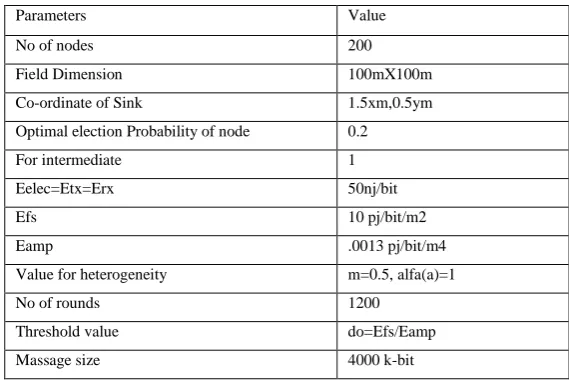
4.1 Simulation Parameter
We take some parameter value to done the simulation comparison between LEACH and MHSEP algorithm. The
parameters used in the simulation are listed in Table.1
TABLE 1: Simulation Parameters Value
Parameters Value
No of nodes 200
Field Dimension 100mX100m
Co-ordinate of Sink 1.5xm,0.5ym
Optimal election Probability of node 0.2
For intermediate 1
Eelec=Etx=Erx 50nj/bit
Efs 10 pj/bit/m2
Eamp .0013 pj/bit/m4
Value for heterogeneity m=0.5, alfa(a)=1
No of rounds 1200
Threshold value do=Efs/Eamp
Massage size 4000 k-bit
The sensor nodes in the network are formed into clusters of different sizes of one, two, three, four and five.
Tround = 0.08 seconds * (Estart / 9 mJ)
Estart: initial energy of the nodes.
Tround: time after which cluster-heads and associated clusters should be rotated.
In this simulation, a total number of 200 nodes were randomly deployed within a space region 100 m x
is randomly distributed in the field. Sink is the destination of each node each node try to send the directly or by
multi-hoping to sink. The initial energy is Eo is set the value of 0.5jule. Let that the size of the data is 4000 kb
that was to be send to base station. This simulation runs on the energy model that was implemented by some
value. The value of each parameter is mention in the table no.6.1. As the Electronic energy (Eelec) is kept the
value 50 nj/bit the same amount of energy is given to receiving electronic energy (Erx) and transitive electronic
energy (Etr). The transmission Amplifier (Eamp) is .0013 pj/bit/m4.We put the value of heterogeneity like the
value of fraction of advanced node m=0.5 and the additional energy factor between advanced and normal nodes
(α) =1 we simulated this model up to 1200 round for each algorithm. Here we describe a threshold (do) which is
calculating the value that a node capability in term of distance if the distance is large then we used the
multi-hoping in that particular cluster head and if it is nearest to sink then it can send the packet data directly. It also
describe the value of a node in the of energy and distance if energy is not enough to send the packet to sink so it
will send to its neighbor node.
This can be describing as formula;
do=Efs/Eamp
equation (5)
4.2 Analysis of Leach Algorithm Simulation
The fig.2. show the area of 100mX100m with 200 node .There is random selection of cluster head between the
node, each round there is selection of 5 % of node as cluster head they aggrades the data form node and send to
base station in this process the dissipation of energy is increase and after losing all the energy the node become
dead. In this plot at a rand time after 200 round we take a snap shot. The green color circle is the normal node,
the black color sign of plus is the advanced node having the extra energy in the random field. The yellow color
triangle is the dead node all the energy of this node is dissipated. The green color circle with black dot is the
cluster head. The boxes of line are clusters.
4.2.1 Average Energy of Node vs. No of Round
There is another graph (fig.3) of leach plot between no. of round and the average energy of node. Its show that
in increasing the no of round the average energy of each node is dissipated more. Its consume the energy during
the transmission of data form node to cluster head as well as cluster head to base station the plot show this
clearly. At 100th round almost node has minimum energy.
Fig.3. Average Energy of Node Fig.4. No. of Dead Node
4.2.2 No of Dead Node vs. No of Round
The individual graph between the no of node die per 100 rounds is shown below fig.4. this plot show the node
are die sudden after a time period of round is the no dead nodes are increase according to the round of
simulation is increase. Approximately 82 to 85 nodes are dead in the starting 100 round in leach algorithm.
4.3 Analysis of MHSEP-Algorithm Simulation
The parameters having the same value in MHSEP algorithm as LEACH. At some random time the plot of
MHESP algorithm are shown in the fig.5. There is the area of 100mX100m with the random distributed node
both the node advanced as well as normal node. The normal node are hallow circle and the blue color plus sign
are the advanced node. Red color big dot is the dead node. The random line boxes are the cluster and the circle
Fig.5. Plot of MHSEP After 1200 Round Fig.6. Average Energy of Node vs. Round Number
4.3.1 Average Energy of Node vs. No of Round
This plot clearly shows the relation between the average energy of node and no of round. In this plot the energy
of average node are dissipated but the rate of dissipate is very slow. As the no of round increase the average
energy decease. The decrease in energy is constantly followed in fig.6.
4.3.2 No of Dead Node vs. No of rounds
We take the starting 100 round and show the simulation. In the starting 100 round the node dead in MHSEP
algorithm is zero. They are more energy efficient then other and no any node is dying in starting 100 round.
Fig.7. No. of Dead Node vs. Round no. in MHSEP
V. SIMULATION RESULT
5.1. Comparison
Both the algorithm are simulate at the same parameters and value. The energy consumption model is different.
The proposed method improved the performance of the system network is seen by the result. Now we compare
implemented beautifully and there result is shown in graph. Now we compare both also through simulation on
the basis of dead node per round and average energy dissipation per round in both LEACH and Improved
LEACH or MHSEP.
5.1.1 Compare on the Basis of Average Energy
In Fig.8 the result of improved method MHSEP are pictured, both the plot is on the same plane and same
parameters. Average energy decline with respect to no. of round are increase because to transmit the data from a
cluster node to cluster head and after sink is a very energy consuming process. Our proposed method improved
the energy efficiency by increasing the average energy of node in the system and prolongs the life cycle of
system. Where the leach result shows that there more than 90 percent of node lose their energy in starting 200
round this show that the through put of the LEACH very poor as compared to the MHSEP. MHSEP not only
dissipated the node energy but also it can maintain the waste of extra energy. After completing the 1200 round
the average energy of system are maintained. The stability period of MHSEP system is increase as compared to
LEACH because the dissipated is slow.
Fig.8. Average Energy of LEACH and MHSEP Fig .9.No of Dead Node in Leach and MHSEP
5.1.2 Compare on the Basis of Dead Node
Fig.9. is the plot of two algorithms LEACH and our proposed method MHSEP; it is plotting between the
parameters of no of node dead with respect to increase in no of round. At the x-axis it shows the no of round at y
direction assuming no dead node. These result are the simulation in Mat lab and a clarification are shown that
proved that our proposed method is fulfill our condition of stability period, the stability period is defined as the
period before the death of first node in system network. In two line graph violate color, and green color
respectively. Leach plot are became early unstable because there node are die very soon after 20-30 round are
after that after that they continuously die at the time period are increased, where as the MHSEP the dead of node
are constant more than 700 round, this period increase stable period very much as compared to the LEACH
more than 20 time. The increased stable period is the achievement of MHSEP because the system life time is
5.3 Result Discussion
Our simulation result are achieved they show that MHSEP Algorithm is better LEACH in performance. We
summarize our general observation:
In wireless sensor network of heterogeneous LEACH going to unstable operation soon, it is very sensitive
to such heterogeneous.
Our MHSEP protocol successful extends the stable region by being aware of heterogeneity. Due to extend stability, the through put of SEP is also higher than the current LEACH. MHSEP is using the multi-hoping so that the energy consume due to large distance are less.
VI. CONCLUSION AND FUTURE WORK
In this paper an energy-efficient multi-hop hierarchical Stable Election Protocol (MHSEP) is improve the
performance of wireless sensor networks, such as energy balancing and reduction, lifetime elongation. The
simulation compares result show that after 1200 round the average energy of network in MHSEP is higher than
the LEACH. The no. of node die in round is less at same round. MHSEP selects those nodes with the highest
residual energy level and weighted election probabilities to act as cluster heads. In each sector, we adopt a
multi-hop communication protocol between normal nodes and cluster head to reduce the cost of long distance
transmission. MHSEP can make a tradeoff between the two criteria of the distance and the residual energy
during the period of the establishment of multi-hop route.
This Paper work, will help the sensor devices to prolong the life of system like as the sensors device used for
area monitoring; it can be helpful in multi-media devices batteries life, through multi-hoping concept the system
failure problem is reduced, the stable period of the system is increased so that the information sharing is not
interrupted due to loss of a single node quickly, this algorithm help to send the huge data from by compress
method and save data as well as batteries.
We can extend MHSEP to deal with clustered sensor networks with more than two levels of hierarchy and more
than two types of nodes with unequal initial energy.
VII. ACKNOWLEDGEMENT
Author, Mr. Mukesh Kushwaha thanks guide, Prof. (Dr.) Bhawna Mallick, Dean Academics and HOD (CSE),
who has the attitude and the substance of a genius and Assistant Prof. Rajkumar Singh Rathore and Assistant
Prof. Sanjay Kumar they support me at every moment of time during research work.
REFERENCES
[1]. M.Sheik Dawood, N.Kaniamudham, M.Thalaimalaichamy.”Study of Energy Efficient Clustering
Algorithm for Wireless Sensor Networks”, International Journal of Emerging Research in Management
&Technology, December 2012.
[2]. A.P.Abidoye, N.A. Azeez,” UDCA: Energy Optimization in Wireless Sensor Network Using Uniform
Distributed Clustering Algorithms”, at Research Journal of Information Technology 2011.
[3]. Bhaskar Krishnamachari, Tutorial Presented at the Second International Conference on Intelligent Sensing
[4]. Krishna M. Sivalingam, Tutorial: Wireless Sensor Networks, University of Maryland, Baltimore County
(UMBC), November 2005.
[5]. Lin Shen and Xiangquan Shi, “A Location based clustering algorithm for wireless sensor networks”,
International Journal of Intelligent Control and Systems, vol. 13, No. 3, 208-213, September 2008
[6]. W.R. Heinzelman, A. Chandrakasan, and H. Balakrishnan, “Energy-efficient Communication Protocol for
Wireless Micro sensor Networks”, in IEEE Computer Society Proceedings of the Thirty Third Hawaii
International Conference on System Sciences (HICSS '00), Washington, DC, USA, Jan. 2000, vol. 8.
[7]. W.R. Heinzelman, A. Chandrakasan, and H. Balakrishnan, “An Application-Specific Protocol
Architecture for Wireless Micro sensor Networks” in IEEE Transactions on Wireless Communications
(October 2002), vol. 1(4).
[8]. Georgios Smaragdakis Ibrahim Matta Azer Bestavros,” SEP: A Stable Election Protocol for clustered
heterogeneous wireless sensor networks”, Technical Report BUCS-TR-2004-022. Computer Science
Department Boston University.
[9]. Boregowda S.B., Hemanth Kumar A.R. Babu N.V, Puttamadappa C., and H.S Mruthyunjaya.” UDCA: An
Energy Efficient Clustering Algorithm for Wireless Sensor Network”, World Academy of Science,
Engineering and Technology 72 2010.
[10].Meenkhshi Sharma and Anil Kumar. Shaw,” Transmission Time and Throughput analysis of EEE
LEACH, LEACH and Direct Transmission Protocol: A Simulation Based Approach”, Advanced
Computing: An International Journal (ACIJ), Vol.3, No.5, September 2012.
[11].Mahmood Ali and Sai Kumar Ravula.” Real-Time Support and Energy Efficiency In wireless sensor
network”, Technical report, January, 2008.
[12].Ted Herman,” A distributed TDMA Slot Assignment algorithm for Wireless Senor Network”, LRI –
CNRS UMR 8623 & INRIA Grand Large, Universities Paris-Sud XI, France, 2004
[13]. C. Intanagonwiwat, R. Govindan, and D. Estrin, "Directed diffusion: A scalable and robust communication
paradigm for sensor networks", Proceedings ACM MobiCom'00, Boston, MA, Aug.2000, pp. 56-67.
[14].Jin Wang1, Xiaoqin Yang1, Yuhui Zheng1, Jianwei Zhang2 and Jeong-Uk Kim3,” An Energy-Efficient
Multi-hop Hierarchical Routing Protocol for Wireless Sensor Networks” International Journal of Future
Generation Communication and Networking Vol. 5, No. 4, December, 2012.
Author’s Profile
Mukesh Kushwaha (Greater Noida, 05/02/1990) received the B.Tech degree in computer
science and engineering from Uttar Pradesh Technical University, Lucknow, Uttar Pradesh,
India in 2011 and pursuing M.Tech in Galgotia’s college of engineering and technology
Greater Noida.(UPTU, LUCKNOW)Uttar Pradesh, India. He has the area of interest are
Wireless Sensor Network, Mobile computing, Data communication Network. He scores 87