MOVING OBJECT DETECTION USING BACKGROUND SUBTRACTION AND SHADOW REMOVAL FROM VIDEO

MOVING OBJECT DETECTION USING

BACKGROUND SUBTRACTION AND SHADOW

REMOVAL FROM VIDEO

Chethan M N

, S K Uma

, B Ramachandra

1

M.Tech student, Dept. of Computer science and engineering, PESCE Mandya, India

2

Assistant Professor, Dept. of Computer science and engineering, PESCE Mandya, India

3

professor and HOD, Dept. of Electrical and electronics engineering, PESCE Mandya, India

ABSTRACT

Surveillance systems are widely used in various fields in recent years. To detect a moving object, a surveillance system utilizes background subtraction, which consists of obtaining a mathematical model of the static background and comparing it with every new frame from the video sequence. Background subtraction is commonly used to detect foreground objects in video surveillance. Traditional background subtraction methods are usually based on the assumption that the background is stationary. However, they are not applicable to dynamic background, whose background images that change over time. This paper proposes an adaptive Local-Patch Gaussian Mixture Model (LPGMM) as the dynamic background model for detecting moving objects from video with dynamic background.The shadow casted by the moving object is also detected. The shadow makes it difficult to detect the exact shape of object and to recognize the object. Therefore, the accurate detection of its exact shape by removing shadows have great influence on the performance of subsequent steps such as tracking, recognition, classification, and activity analysis. A cascading chromaticity difference estimator, brightness difference estimator, and spatial analysis are explored to discriminate the shadow and the moving object.

Keywords -

Background Subtraction, Local-Patch Gaussian Mixture Model, Moving Object

Detection, Dynamic Background,

Shadow Removal, Chromaticity Difference,

Brightness Difference, Spatial Analysis

I. INTRODUCATION

Moving object detection is one of the essential tasks in many computer vision applications, such as traffic

monitoring and miltary. A typical and an efficient approach used to achieve such tasks is background subtraction.

The idea behind background subtraction is to compare the current frame with a reference background model

(reference model) which is learned and maintained in the background for a long time. Much effort has been

devoted in developing efficient methods of moving object detection using background subtraction. Some of them

estimated the probabilities of individual pixels belonging to background by using Gaussian Mixture Models

(GMMs) [1] or labeled each pixel as foreground or background by Markov Random Fields (MRFs) [2].An

improved GMM learning algorithm [3] was proposed to select an appropriate number of components for each

pixel on-line, thus fully adapting to the scene. Elgammal et al. [4] proposed to utilize a general nonparametric

kernel density estimation technique to build background model for detecting foreground objects. These methods

case of the dynamic scenes, which include repetitive motions like moving car, people walking etc. Several

block-based methods were developed to overcome such problems, which usually divide an image into blocks and

calculate block correlation [5] or block-specific features, such as the local binary pattern [6] histogram. However,

these block-based approaches allow only coarse detection of the moving objects. Some recent methods proposed

for dynamic background subtraction utilized not only the temporal information of a single pixel but also the

spatial information of neighboring pixels. Li et al. [7] extracted foreground objects from a complex video under

the Bayes decision framework. A Bayes decision rule was employed for classification of background and

foreground from a general feature vector. Sheikh and Shah [8] also utilized a Bayes rule to build the background

model based on an MRF framework to enforce the spatial constraint and obtained better results. Zhang et al. [9]

proposed a spatial-temporal nonparametric background subtraction method to effectively handle dynamic

background subtraction by modeling the spatial and temporal variations simultaneously.

In this paper, we propose a foreground detection algorithm from dynamic background videos. First, we propose a

Local-Patch Gaussian Mixture Model (LPGMM) which is the extension of the GMM to represent local spatial

distribution for each pixel. Fig.1 gives the foreground object extraction using LPGMM. Foreground object

extraction have two phases. 1.Training phase 2.Testing phase. In training phase using image sequence build

LPGMM background model (reference model). In testing phase new image sequence is compared with reference

background model. If the observed pixel is matched to a Gaussian distribution and the mean difference falls

within 2.5 times the corresponding standard deviation, then that pixel is classified as background and updated as

background. Fig.1 shows the flow chart of the system. The shadow casted by the moving object is also detected.

The shadow makes it difficult to detect the exact shape of object and to recognize the object. Therefore, the

accurate detection of a moving object and the acquisition of its exact shape by removing shadows have great

influence on the performance of subsequent steps such as tracking, recognition, classification, and activity

analysis. Rest of this paper is organized as follows. In Section 2 LPGMM background modeling method. Section

3shows shadow removal method. Section 4 we show some experimental results. Section 5 shows conclusion.

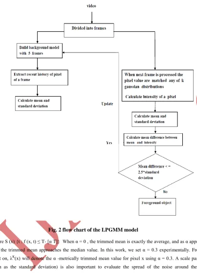
II. LPGMM BACKGROUND MODEL

The proposed method is a foreground object extraction technique for video surveillance system. Most of the

traditional object detection approaches uses background is stationary. We consider the problem that the

background is dynamic and usually change quickly overtime. Fig. 2 flow chart of the LPGMM model

Take 1st frames(ex.5 frames) of the video as a training data for building the background model.

Extract recent history of a pixel (intensity and mean standard deviation) from a frame.

A. Intensity.

B. Mean and Standard deviation.

2.1 Intensity

Let the recent history of a pixel be {X1,...,XN}, which is modeled by a mixture of K Gaussian distributions,

and X be an intensity vector for R, G and B color channels. At time t, the probability density function at

observing pixel value Xt is given by

(1)

Where η is the Gussian probability density function which is defined as

(2)

The main difference between LPGMM and GMM [1] is that Xt,µt and σt for each pixel are vectors formed from

observations from its local neighborhood instead of scalar values.

The covariance matrix ∑ is defined as:

∑ = (3)

Where d x d is the local patch size for each pixel, and σi denote the standard deviation for the i th

pixel. Let ft(x,y)

be the intensity value of the observed pixel; mt(x,y) and st(x,y) are the corresponding mean and standard

deviation of the background model at time t in the original GMM [1]. For each observed pixel, set a window

around the pixel as the center. Let the window size be d x d, we can extend the original Xt that is a single value

in the original GMM model to a d2-dimensional vector for each observed pixel as follows:

T

(4)

Where d′ = (d-1)/2 is assumed to be an integer without loss of generality.

2.2 Mean and standard deviation

The mean µt and standard deviation σt are extended to d2-dimensional vectors for each background pixel, i.e.

(5)

These vectors represent the local spatial information in a local neighborhood for each pixel. When a new frame

is processed, we first check if the color values for each pixel are matched to any of the K Gaussian distributions.

Then mean difference between Xt(x,y) and µt(x,y) is computed as follows:

D(X

(x,y),µ

(x,y)) = ∑

| f

(x+i ,y+j) – m

(x+i,y+j)|

If the observed pixel is matched to a Gaussian distribution and mean difference falls within 2.5 times the

corresponding standard deviation, then that pixel is classified as background. The equation to classify the

pixel is given by

D(X

(x,y),µ

(x,y)) ≤ 2.5∑

σ

(x+i ,y+j)

In the updating process, we update σt(x,y) and µt(x,y) for those pixels to classify background as follows:

(10)

Where

σ

﴾x ,y﴿

-

III. SHADOW REMOVAL

To remove shadow 1st foreground object is extracted by using background subtraction method, then shadow

removal technique is used. A cascading chromaticity difference estimator, brightness difference estimator, and

spatial analysis are explored to discriminate the shadow and the moving object. Estimated the background by

using a metrically trimmed mean and also including a local spatial coherence for foreground detection.

Let us denote the position of a pixel x = (x, y), and the intensity of each pixel p(x) is expressed as I (x), which is

defined as follows:

I (x) = [I R (x), I G (x), I B (x)]T (11)

Where I R(x), I G(x) and I B(x)denote the intensity of the red, green, and blue component, respectively. For

notational simplicity, we will use superscript K representing R,G or B. Suppose [I1(x), I2 (x),…, IT (x)] be T

image frames used in the training stage, and M(x) be the image containing the temporal median of each pixel x.

For 0 ≤ α < 1, the α -metrically trimmed mean ( x) of each RGB component for each pixel is obtained by

computing the temporal average of (x) ,disregarding the largest [αT ] deviations from the median (here, [. ]

denotes the greatest integer function). Formally, let us consider an ordering of the differences | (x)-Mk (x)| and

define an integer function 1 ≤ f (x,t) ≤ T that returns theposition of | (x)-Mk (x)| in such ordering. The α

-metrically trimmed mean is ( x) given by

Fig. 2 flow chart of the LPGMM model

Where S (x) {t : f (x, t) ≤ T- [α T]} When α = 0 , the trimmed mean is exactly the average, and as α approaches one, the trimmed mean approaches the median value. In this work, we set α = 0.3 experimentally. From this point on, λK_{(x) will denote the α -metrically trimmed mean value for pixel x using α = 0.3. A scale parameter}

(such as the standard deviation) is also important to evaluate the spread of the noise around the actual

background value. A robust scale estimator is given by the mean absolute deviation (MAD), defined as

MAD

(x)=median

{| (x)-M

(x)|}

If additive Gaussian noise is assumed, the relation σ K_{(x) =1.4826MAD}K_{(x) provides an estimate of the standard}

deviation of each RGB component for each pixel. Pixels belonging to the foreground are probably far from the

appear in blobs, so we analyze a small neighborhood around each pixel. A pixel x is assigned to the foreground

if

∑

w(u) | (x) - λ

(u)| > h ∑

w(u)σ

(u)

Where Ω (x) is a small neighborhood centered at x, w(u) is a weighting mask for each pixel u = (u,v), and h controls the maximum allowed deviation from the mean w.r.t. the standard deviation. In this work, w is the

weighted average mask, whose central point has weight 4, vertical and horizontal neighbors weight 2, and

diagonal neighbors weight 1.We set a 3×3 neighborhood for Ω and h = 3. In practical applications, the detection

of foreground pixels using [3] may produce some isolated pixels, or holes in the interior of valid objects. To

overcome this problem, we apply sequentially an opening and a closing morphological operator.

Feature extracted for shadow removal

A. Chromaticity difference estimator.

B. Brightness difference estimator.

C. Spatial analysis for shadow verification.

The drawback of background subtraction techniques is the undesired detection of shadows as foreground

objects. A cascading process is proposed to detect shadows from foreground pixels. We discard the local

relation estimator and change the strategy of the spatial adjustment step. The shadow detection process is

described as follows.

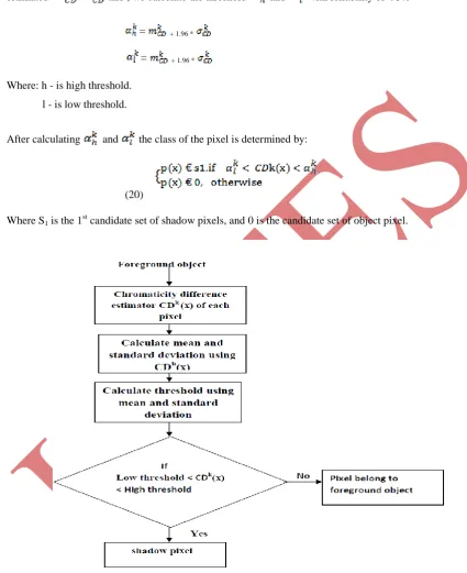
A.Chromaticity difference estimator

The Fig.3 shows the flow chart of Chromaticity difference estimator. To discriminate the shadow pixel and the

object pixel, we define the chromaticity difference CDk(x) as follows:

CDk(x) = (x) / ||Is (x)|| - (x) / ||Ib(x)|| (15)

Where the subscripts s and b represent the shadow and the background respectively. ||Is (x) and Ib(x)|| are the

norm of Is(x) and Ib(x) respectively. For every pixel x in the set of moving pixels, we calculate CDK (x).

According to the assumptions in [7], CDK(x) of the shadow pixels has Gaussian distribution, and its mean is

close to zero, because shadow pixel is darker than background. So, a pixel which is brighter than the background

cannot be a shadow pixel, and it conclude that it is a moving object pixel. CDK(x) of the moving object pixel has

an unknown distribution that depends on the object. Thus, we can determine that a pixel is a moving object pixel

if CDK(x) is far from zero. To reduce computation, we only use pixels which satisfy the following condition.

-0.2 ≤ CDK(x) ≤ 0.2

While estimating the mean and the standard deviation .Then, and can be estimated as

follows:

= 1/ N

∑

CD

(x)

( )2

= 1/ N

∑ (CD

(x)

-

)

(17)

Where NM is the set of pixels which satisfy − 0.2 ≤ CD K

(x) ≤ 0.2 in the set of moving pixels. Using the

estimated and , we calculate the threshold and with reliability of 95%

= + 1.96 * (18)

= + 1.96 * (19)

Where: h - is high threshold.

l - is low threshold.

After calculating and the class of the pixel isdetermined by:

(20)

Where S1 is the 1 st

candidate set of shadow pixels, and 0 is the candidate set of object pixel.

Fig. 3 Flow chart of Chromaticity difference estimator

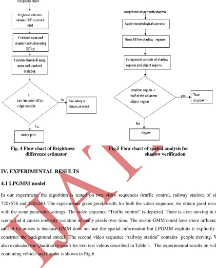
B. Brightness difference estimator

After extracting chromaticity difference estimator, there still exist many moving object pixels in the 1st

candidate set of shadow pixels. This shadow pixels can be removed by Brightness difference estimator. The

The brightness difference estimator separates moving object pixels from the 1st candidate set of shadow pixels

using brightness difference BDK (x) of all pixels in the 1st candidate set of shadow pixels. BDK (x) can be

defined as

BDk(x) = /

(21)

The distribution of BDK (x) of the shadow pixels is Gaussian such that the mean is and the standard

deviation is . We estimate and as follows:

= 1/ N

∑ BD

(x)

p(x)€M

Where NS is the number of pixels in S1.Using the estimated and , we calculate the threshold and

as follows: with reliability of 95%.

= + 1.96 * (23)

= - 1.96 * (24)

Where: h - is high threshold, l - is low threshold.

After calculating and , the class of the pixel is determined by

(25)

Where S2 is the 2nd candidate set of shadow pixels, and 0 is the candidate set of object pixels.

C. Spatial Analysis for Shadow Verification

By the previous two estimators, the set of moving pixels are divided into the 2nd candidate set of shadow pixels

and the candidate set of object pixels. However, two types of shadow detection errors may commonly occur,

namely shadow detection failure and object detection failure. To improve the accuracy of shadow detection, a

post processing spatial analysis is added for shadow confirmation. Then analysis is done to confirm the true

shadows as well as the true objects according to their geometric properties.

The Fig.5 shows the flow chart of spatial analysis for shadow verification. In order to break the weak connection

between shadow regions, we apply an opening morphological operator to the shadow mask. Then a flood-fill

operation is used to fill the holes in shadow regions. The foreground consists of shadow regions and object

regions. If the shadow candidate is a true shadow, less than a half of the boundary should be adjacent to the

boundaries of object regions. Thus we can use the boundary information of a shadow candidate region to

confirm whether the shadow is a true shadow or not. The outer pixels ES of each candidate shadow mask MS can

be calculated as follows:

ES = MS ⊕ SE –MS (26)

Where ⊕ is the dilation operator and ES is the structure element of 3×3 square. If the proportion of object pixels

Fig. 4 Flow chart of Brightness Fig.5 Flow chart of spatial analysis for difference estimator shadow verification

IV. EXPERIMENTAL RESULTS

4.1 LPGMM model

In our experiment, the algorithm is tested on two video sequences (traffic control, railway station) of size

720x576 and 320x240. The experiments gives good results for both the video sequence, we obtain good results

with the some parameter settings. The video sequence “Traffic control” is depicted. There is a car moving in the

scene, and it causes intensity variation of many pixels over time. The reason GMM could have more influences

caused by noises is because GMM does not use the spatial information but LPGMM exploits it explicitly to

construct the background model. The second video sequence “railway station” contains people moving. We

also evaluated the Qualitative result for two test videos described in Table 1. The experimental results on video

containing vehicle and human is shown in Fig 6.

Test video Method TP FN TPR

Traffic control

LPGMM 50 10 83.3

Railway station

LPGMM 48 12 81.6

We have tested with 1second video for traffic control and railway station we have calculated the sensitivity

(TPR- true positive rate) for the above said videos using formula

TPR ═ TP ⁄ ( TP + FN) (27)

Where: TP – True Positive, FN- False Negative

(a,1) (a,2)

(b,1) (b,2)

(c,1) (c,2)

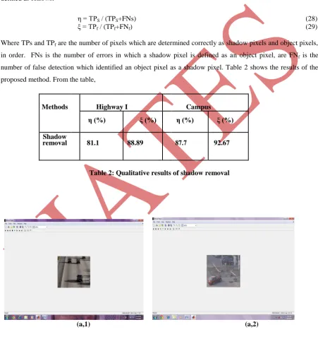
4.2 Shadow removal

The proposed algorithm is tested on two video sequences (Highway I, Campus) which can be downloaded from

http://cvrr.ucsd.edu/aton/shadow. First 100 frames are used for background training for Highway I sequence;

while for Campus sequence, From the Fig 7 shows the snapshot of shadow removal method.

To evaluate the performance of the proposed shadow removal method quantitatively, we calculate the shadow

detection rate and shadow discrimination rate. The shadow detection rate η and shadow discrimination rate ξ are

defined as follows:

η = TPS / (TPS+FNs) (28)

ξ = TPf / (TPf+FNf) (29)

Where TPs and TPf are the number of pixels which are determined correctly as shadow pixels and object pixels,

in order. FNs is the number of errors in which a shadow pixel is defined as an object pixel, are FNf is the

number of false detection which identified an object pixel as a shadow pixel. Table 2 shows the results of the

proposed method. From the table,

Table 2: Qualitative results of shadow removal

(a,1) (a,2)

Methods Highway I Campus

η (%) ξ (%) η (%) ξ (%)

Shadow

removal 81.1 88.89 87.7 92.67

(b,1) (b,2)

Fig7 (a) input frame (b) frame after removing shadow

V.

CONCLUSION

In this paper, we proposed a LPGMM model is used detect moving object from surveillance videos with

dynamic background, which consider the local spatial information for each pixel. This approach is used for

object detection with background subtraction and shadow removal in the RGB color space. For background

subtraction, the metrically trimmed mean is used as a robust estimate of the background model, and the MAD

(mean absolute deviation) is adopted as a scale estimate. The shadow and the moving object are discriminated

by cascading two estimators which use the properties of chromaticity and brightness. The spatial information is

utilized to verify the true shadow regions. Our experimental results show the good performance of the proposed

method. For future work, texture and edge information will be adopted as features to further improve the

shadow detection accuracy. Classification method can be applied after the extraction of foreground object for

further analysis of moving object whether it is human or vehicle.

References

[1] C. Staufer, W.E.L. Grimson, “Adaptive background mixture models for real-time tracking,” CVPR, Vol. 2, pp. 246-252,1999.

[2] N. Paragios and V. Ramesh, “A MRF-based approach for real time subway monitoring,” CVPR, vol. 1, pp. 1034-1040, 2001

[3] Z. Zivkovic and F. van der Heijden, “Recursive unsupervised learning of finite mixture models,” IEEE Trans. PAMI, Vol.26, No.5, pp. 651–656, 2004.

[4] A. Elgammal, D. Harwood, and L. Davis, “Non-parametric model for background subtraction,” ECCV, 2000.

[5] T. Matsuyama, T. Ohya, H. Habe, “Background subtraction for non-stationary scenes,” ACCV, pp. 662–667, 2000.

[6] M. Heikkila and M. Pietikainen, “A texture-based method for modeling the background and detecting moving objects,” IEEE Trans. PAMI, Vol. 28, pp. 657-662, 2006.

[8] Y. Sheikh and M. Shah, “Bayesian modeling of dynamic scenes for object detection,” IEEE Trans. PAMI, Vol. 27, pp. 1778-1792, 2005.

[9] S. Zhang, H. Yao, and S. Liu, “Spatial-temporal nonparametric background subtraction in dynamic scenes,”

ICME, 2009

[10]L. Cheng and M. Gong, “Real-time background subtraction from dynamic scenes,” ICCV, 2009.

[11]S.-S. Huang, L.-C. Fu, and P.-Y. Hsiao Region-level motionbased background modeling and subtraction using mrfs,” IEEE Trans. Image Processing, vol. 16, no. 5, pp. 1446 –1456, 2007.

[11] E. Salvador, A. Cavallaro, and T. Ebrahimi, "Cast shadow segmentation using invariant color features," Computer Vision and Image Understanding, vol. 95, pp. 238-259, August 2004.