:THE COSMOLOGICAL OTOC:
Formulating new cosmological micro-canonical correlation
functions for random chaotic fluctuations in
Out-of-Equilibrium Quantum Statistical Field Theory
Sayantan Choudhury
1Quantum Gravity and Unified Theory and Theoretical Cosmology Group, Max Planck Institute for Gravitational Physics (Albert Einstein Institute),
Am Mu¨hlenberg 1, 14476 Potsdam-Golm, Germany.
Email: [email protected]
Abstract
The out-of-time-ordered correlation (OTOC) function is an important new probe in quan-tum field theory which is treated as a significant measure of random quanquan-tum correlations. In this paper, with the slogan “Cosmology meets Condensed Matter Physics” we demon-strate a formalism using which for the first time we compute the Cosmological OTOC during the stochastic particle production during inflation and reheating following canoni-cal quantization technique. In this computation, two dynamicanoni-cal time scanoni-cales are involved, out of them at one time scale the cosmological perturbation variable and for the other the canonically conjugate momentum is defined, which is the strict requirement to define time scale separated quantum operators for OTOC and perfectly consistent with the general definition of OTOC. Most importantly, using the present formalism not only one can study the quantum correlation during stochastic inflation and reheating, but also study quantum correlation for any random events in Cosmology. Next, using the late time exponential decay of cosmological OTOC with respect to the dynamical time scale of our universe which is associated with the canonically conjugate momentum operator in this formalism we study the phenomena of quantum chaos by computing the expression for Lyapunov spectrum. Further, using the well known Maldacena Shenker Stanford (MSS) bound, on Lyapunov exponent,λ≤2π/β, we propose a lower bound on the equilibrium temperature, T = 1/β, at the very late time scale of the universe. On the other hand, with respect to the other time scale with which the perturbation variable is associated, we find decreasing but not exponentially decaying behaviour, which quantifies the random quantum correla-tion funccorrela-tion at out-of-equilibrium. We have also studied the classical limit of the OTOC check the consistency with the large time limiting behaviour of the correlators. Finally, we prove that the normalized version of OTOC is completely independent of the choice of the preferred definition of the cosmological perturbation variable.
Keywords: Cosmology beyond the standard model, Quantum Dissipative Systems, Stochastic Processes, Effective Field Theories.
Contents
1 Introduction 2
2 Formulation of OTOC in Cosmology 16
2.1 General remarks on OTOC 16
2.2 Eigenstate representation of OTOC in quantum statistical mechanics 19
2.3 Constructing OTOC in Cosmology 23
2.3.1 For massless scalar field 30
2.3.2 For partially massless scalar field 36
2.3.3 For massive scalar field 37
3 Quantum micro-canonical OTO amplitudes and OTOC in Cosmology 40
3.1 Computational strategy 41
3.2 Classical mode functions in Cosmology 43
3.3 Quantum mode function in Cosmology 47
3.4 Canonical quantization of cosmological Hamiltonian: Classical to quantum
map 50
3.5 Cosmological two-point and four-point “in-in” OTO micro-canonical
ampli-tudes 51
3.5.1 OTOC meets Cosmology 51
3.5.2 Fourier space representation of the commutator bracket: Application
to two-point OTOC 53
3.5.3 Fourier space representation of square of the commutator bracket
Application to four-point OTOC 56
3.6 Cosmological thermal partition function: Quantum version 61
3.6.1 Quantum vacuum state in Cosmology 61
3.6.2 Quantum partition function in terms of rescaled field variable 61
3.6.3 Quantum partition function in terms of curvature perturbation field
variable 62
3.7 Trace of two-point “in-in” OTO amplitude for Cosmology 64
3.8 OTOC from regularised two-point “in-in” OTO micro-canonical amplitude:
rescaled field version 65
3.9 OTOC from regularised four-point “in-in” OTO micro-canonical amplitude:
curvature perturbation field version 67
3.10 Trace of four-point “in-in” OTO amplitude for Cosmology 69
3.11 OTOC from regularised four-point “in-in” OTO micro-canonical amplitude:
rescaled field version 70
3.11.1 Without normalization 70
3.11.2 With normalization 74
3.12 OTOC from regularised four-point “in-in” OTO micro-canonical amplitude:
curvature perturbation field version 75
3.12.2 With normalization 75
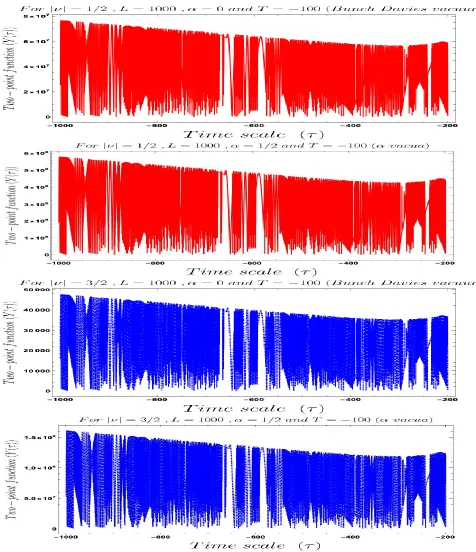
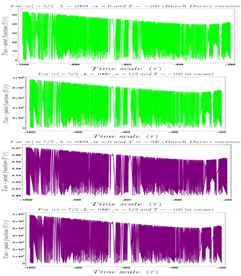
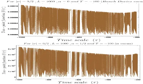
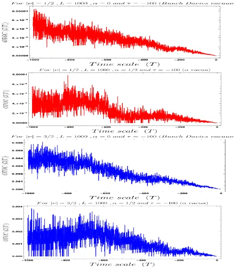
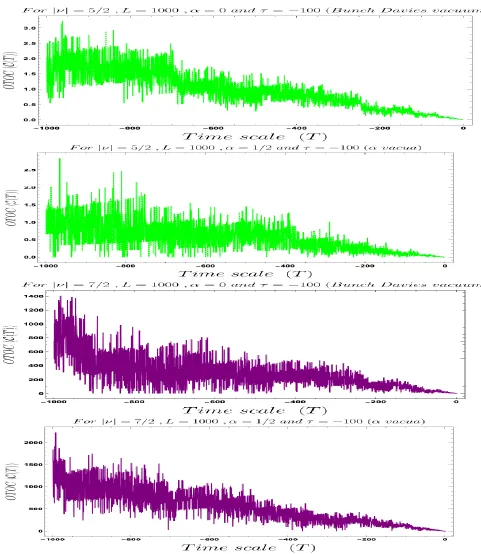
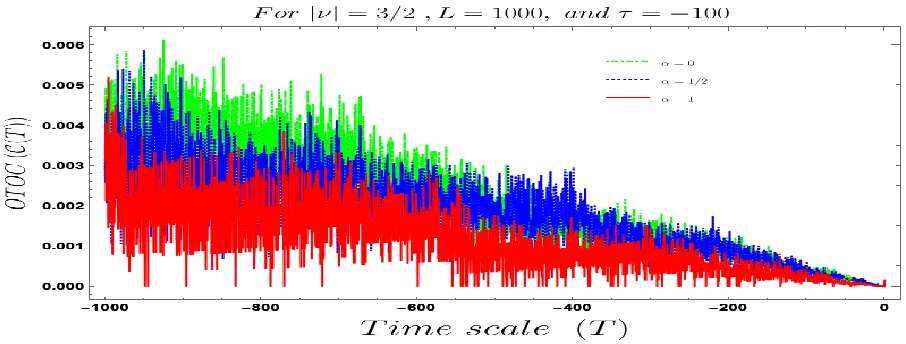
4 Numerical results I: Interpretation of two-point micro-canonical OTOC
in Cosmology 78
5 Numerical results II: Interpretation of four-point micro-canonical OTOC
in Cosmology 93
6 Lyapunov spectrum and quantum chaos in Cosmology 98
7 Numerical results III: Interpretation of cosmological Lyapunov spectrum103
8 Classical limit of micro-canonical OTO amplitudes and related OTOC in
Cosmology 108
8.1 Computational strategy 108
8.2 Classical limit of cosmological two-point “in-in” OTO micro-canonical
am-plitudes 109
8.3 Classical limit of cosmological four-point “in-in” OTO micro-canonical
am-plitudes 111
8.4 Cosmological micro-canonical partition function: Classical version 114
8.4.1 Classical micro-canonical partition function in terms of rescaled field
variable 114
8.4.2 Classical micro-canonical partition function in terms of curvature
perturbation field variable 115
8.5 Classical limit of cosmological two-point micro-canonical OTOC: rescaled
field version 116
8.6 Classical limit of cosmological two-point micro-canonical OTOC: curvature
perturbation field version 118
8.7 Classical limit of cosmological four-point micro-canonical OTOC: rescaled
field version 118
8.7.1 Without normalization 118
8.7.2 With normalization 121
8.8 Classical limit of cosmological four-point micro-canonical OTOC: curvature
perturbation field version 121
8.8.1 Without normalization 121
8.8.2 With normalization 122
9 Summary and Outlook 123
A Asymptotic behaviour of the cosmological mode functions 129
B WKB solution of the cosmological mode functions for time dependent
C Quantum two-point OTO micro-canonical amplitudes for Cosmology 140
C.1 Definition of micro-canonical OTO amplitude ˆ∆1(k1,k2;τ1, τ2) 140
C.2 Definition of micro-canonical OTO amplitude ˆ∆2(k1,k2;τ1, τ2) 140
D Quantum four-point OTO micro-canonical amplitudes for Cosmology 142
D.1 Definition of micro-canonical OTO amplitude Tb1(k1,k2,k3,k4;τ1, τ2) 142
D.2 Definition of micro-canonical OTO amplitude Tb2(k1,k2,k3,k4;τ1, τ2) 143
D.3 Definition of micro-canonical OTO amplitude Tb3(k1,k2,k3,k4;τ1, τ2) 144
D.4 Definition of micro-canonical OTO amplitude Tb4(k1,k2,k3,k4;τ1, τ2) 145
E Computation of classical limit of four-point “in-in” OTO micro-canonical
amplitudes for Cosmology 146
F Computation of quantum micro-canonical partition function in
Cosmol-ogy 149
F.1 Quantum micro-canonical partition function in terms of rescaled field variable149
F.2 Quantum micro-canonical partition function in terms of curvature
pertur-bation field variable 150
G Computation of classical micro-canonical partition function in
Cosmol-ogy 152
G.1 Classical micro-canonical partition function in terms of rescaled field variable152
G.2 Classical micro-canonical partition function in terms of curvature
perturba-tion field variable 153
H Computation of the trace of the two-point amplitude in micro-canonical
OTOC 154
I Computation of the trace of the four-point amplitude in micro-canonical
OTOC 156
J Time dependent two-point amplitude in micro-canonical OTOC 162
K Time dependent four-point amplitudes in micro-canonical OTOC 164
K.1 Computation of I1(τ1, τ2) 165
K.2 Computation of I2(τ1, τ2) 180
K.3 Computation of I3(τ1, τ2) 181
K.4 Computation of I4(τ1, τ2) 181
K.5 Computation of I5(τ1, τ2) 182
K.6 Computation of I6(τ1, τ2) 182
K.7 Computation of I7(τ1, τ2) 183
K.8 Computation of I8(τ1, τ2) 183
L Computation of the normalization factor in four-point micro-canonical
OTOC 185
L.1 Normalization factor of four-point micro-canonical OTOC computed from
rescaled field variable 185
L.2 Normalization factor of four-point micro-canonical OTOC computed from
curvature perturbation field variable 189
M Computation of the normalization factor in classical limit of four-point
micro-canonical OTOC 190
M.1 Normalization factor of the classical version of four-point micro-canonical
OTOC computed from rescaled field variable 190
M.2 Normalization factor of the classical version of four-point micro-canonical
OTOC computed from curvature perturbation field variable 192
N Thermal trace operation in terms of wave function of the universe in
Cosmology 194
This work is written in the memory of the great physicist Professor Freeman J. Dyson
with whom I had the chance to meet personally and discuss my work and understandings during my visit at Institute for Advanced Studies (IAS), Princeton for the purpose of
participating at the Workshop on Qubits and Spacetime which happened on the first week of December, 2019. Here I have to acknowledge the strong support from Professor Juan Martin Maldacena, who had invited me for the mentioned prestigious workshop and
also the Max Planck Institute for Gravitational Physics (Albert Einstein Institute), Potsdam, Germany for providing me the financial support to attend this workshop, also
1
Introduction
The out-of-time ordered correlation (OTOC) [1–7] functions in the context of quantum field theory at finite temperature is considered as a very strong probe of any kind of stochasticity, randomness and quantum mechanical chaos in the present day research of theoretical physics. Earlier it was only studied in the various condensed matter systems where out-of-equilibrium phenomena plays significant role. The concept of OTOC was first introduced in the computation of superconductivity to describe the vertex correction of current [9]. But for the past few years theoretical physicist are applying this idea to explore various unknown out-of-equilibrium features of various quantum field theories at finite temperature and in the context of bulk gravitational theories. From the very common understanding one can physically interpret OTOC as a quantum mechanical analogue of the classical version of the sensitiveness against tiny random fluctuations in the initial conditions, and particularly if we get exponential growth in the time dynamics of the OTOC then it is treated as a very strong probe of quantum mechanical chaos 2. In terms of the traditional physics one can think of this concept as the theoretical indicator of the energy gaps, and in that connection it is very interesting to investigate that whether or not the OTOC can be treated as a better probe of stochastic randomness and quantum mechanical chaos at out-of-equilibrium.
To describe this in a more technical way, let us consider two quantum operators X(t) and Y(0), which are separated in time scale and using them OTOC is defined by the following expression [1]:
How to define OTOC? C(t) :≡ −h[X(t), Y(0)]2iβ =−
1 Z Tr
exp (−βH) [X(t), Y(0)]2 ,
(1.1) where the thermal partition function is defined as:
Partion function: Z = Tr [exp (−βH)] where β = 1
T with kB= 1 . (1.2)
Specifically in this context commutator of the two time separated operator in quantum mechanics describes the effect of perturbation by the operator Y on the measurement of the operator X on later time scales and the converse statement is also true here. In this construction, we also assume that these two operators have zero one point functions. Now if we fix these operators as, two canonically conjugate operators i.e. in terms of position operator X(t) = q(t) and momentum operator Y(0) = p(0) for a quantum system, then in the semi-classical limit, one can replace the commutator bracket of these two operators, [q(t), p(0)], will be replaced by the Poisson bracket, i{q(t), p(0)}PB = i(∂q(t)/∂q(0)) (in
2In terms of Schr¨odinger time evolution it is very difficult to describe such quantum phenomena in
the natural unit system, where we take, ~ = 1). For classical system to have chaotic description, (∂q(t)/∂q(0))∼exp(λt), whereλis theLyapunov exponent, which is appearing as an outcome of the sensitiveness of the initial conditions. Consequently, if we compute the expression of OTOC out of these two canonically conjugate quantum operators then it will scale with resopect to time scale as, C(t)∼exp(2λt), to achieve a quantum chaotic description from this set up and here λ is treated as quantum Lyapunov exponent. It is expected from this discussion that, if we can able to quantize the classical chaotic system properly then it can provide a positive numerical value of thequantum Lyapunov exponent
within the framework of OTOC. Following this discussion one can further distinguish between the classical and quantum chaotic system, which comes from the computation of OTOC and the time evolution of this shows that in quantum mechanics OTOC is a quantity which does not grow with the evolutionary time scale of the quantum theory but at the late time scales saturates to a constant value and in this literature this time scale is identified as the Ehrenfest time scale. one can also describe this characteristic time scale a critical scale after which the quantum mechanical wave function of the theory spreads over the whole system under consideration for this description 3
As we have already mentioned in the present day research the concept of OTOC getting more attention due to the fact that, it can be served the purpose of a strong theoretical probe of possible bulk gravitational dual theories, in terms of the framework of AdS/CFT correspondence [10, 11]. One can quote here many many examples to feature the impor-tance of the OTOC’s in the context of AdS/CFT. One of the famous examples are the study of the existence of shock waves in the black hole physics [12–15, 17] which can be described by various types of geometries and this specific study finally led to maximum saturation bound of the quantum version of the Lyapunov exponent (λ), given by the following expression [1]:
M(aldacena) S(henker) S(tanford) bound: λ≤ 2π
β with ~= 1, c = 1, kB = 1 .(1.3)
which is appearing in the expression for OTOCs at finite temperature. This well known bound was established byMaldacena, Shenker, Stanford, which is commonly addressed as
MSS bound on quantum chaos these days [1]. In gravitational paradigm, this saturation bound is physically interpreted as the red shift factor near the black hole event horizon having a finiteHawking temperature. In this description,Sachdev-Ye-Kitaev (SYK)model [16,18–27] is the most famous example at present which can able to saturate theMSS bound
very successfully, which describes the quantum mechanical model of Majorana fermions in presence of infinitely long disorder. In the context ofSYKmodel the saturation of theMSS boundcorresponds to a quantum mechanical description of the black hole paradigm within
3In a very rough sense, very crudely also this characteristic time scale is identified as the transition
the framework of AdS/CFT correspondence. Most significantly, it is important to note that the appearance of quantum Lyapunov exponent in the computation of OTOC allows to consider the connection with the bulk gravitational physics in the quantum mechanical regime by applying the understanding from AdS/CFT correspondence. From the detailed past study in this literature we already know that any bulk gravitational physics which have their own dual description are described by the strongly quantum mechanical description. So from the present discussion it is evident that, to connect this description with the phenomena of quantum mechanical chaotic picture we explicitly need to have an analogous description of quantum Lyapunov exponent, which will mimic the role of the well known
Lyapunove exponentas appearing in the description of chaotic dynamical classical systems and to serve this purpose successfully, OTOC is the only strongest probe which can be treated as the physical discriminator of the classical and quantum mechanical description in the present context of discussion.
which one can explain the origin of previously mentioned scalar and tensor fluctuations, which are treated to be quantum to describe the physics of early universe and for the late time scale it is considered to be classical in nature. These quantum fluctuations are very fundamental objects in the context of Cosmology from which all N-point correlation functions can be computed in Fourier space and these results can be used to probe the physics of early universe as well as to comment on its impact on the present day galaxy and cluster formation in large scale structure non-linear cosmological perturbation theory. Apart from having a great understanding the computation of these correlation functions of the quantum fluctuations at thermodynamic equilibrium, we have till now have a lot of constraints and limitations from the observational probes. From cosmological observations till now we have information regarding the amplitude of the primordial power spectrum from scalar mode fluctuations4 [34] and about its nearly scale invariance feature with
re-spect to momentum scale 5. Additionally, we have information regarding upper bound on
the tensor-to-scalar ratio6 at the cosmological horizon scale from the observational probes. No other information regarding the higher point (three and four-point etc.) cosmological correlation functions are not available till now with significant statistical accuracy which can also be treated as the probe of new physical phenomena through non-Gaussianity in the primordial Cosmology. This implies that, just using the present observational probes one cannot able to distinguish amongst various possible origin of primordial quantum me-chanical fluctuations and rule out models which describes inflationary paradigm within the framework of Cosmology. So one can immediately ask about a questions regarding the possible options left to explore the physics of primordial quantum fluctuations:
• Possibility I:
The first possibility pointing towards the future observational aspects which can be probed by different ongoing and upcoming experiments to verify various theoretical features of primordial Cosmology. The most significant quantity using which it is possible to understand the underlying quantum field theory origin of the primor-dial physics is tensor-to-scalar ratio. Detection of this observable with high statisti-cal accuracy will provide us the information regarding the generation of primordial
4This is actually represent the amplitude of the cosmological two-point correlation function of scalar
mode quantum fluctuations in Fourier space.
5This constraint will helps us to determine the feature of the primordial power spectrum for scalar
modes in all cosmological momentum scales. Till now from observational probes only the information regarding the spectral index (which is represented by the logarithmic derivative of the logarithm of the power spectrum at the cosmological horizon crossing scale) with high statistical accuracy is available. Any further information, such as running and the running of the running of the scalar spectral index are not available with any significant statistical accuracy.
6It represents the ratio of the amplitude of the power spectrum from tensor and scalar modes fluctuation
gravitational waves, which will further confirms the exact origin of the primordial quantum mechanical fluctuations by exactly estimating the scale of inflation. Not only discriminating different frameworks of inflationary paradigm, but also the ex-istence of alternatives to inflationary frameworks i.e. bouncing cosmology, cyclic cosmology, ekpyrotic scenario etc. can also be verified by the confirmation of the primordial gravity waves. The next important quantity within the framework of pri-mordial Cosmology is study the existence of non-Gaussian features in the quantum mechanical fluctuations and the probability distribution profile of its related correla-tion funccorrela-tions. For this purpose the study of bispectrum and trispectrum, which are basically representing the momentum dependent amplitude of the three-point and four-point correlation function are very important. In near future through the up-coming cosmological missions if it is possible to detect these non-Gaussian amplitudes with high statistical accuracy then it is further put more stringent constraint on the primordial physics. This is because of the fact that, the probability distribution of such quantum fluctuations in the primordial universe is almost following Gaussian profile and a small but significant deviation from such Gaussianity will be extremely helpful to discriminate amongst various possible theoretical models of inflation which can able to generate significant amount of non-Gaussian amplitude in the context of three-point and four-point correlation functions. We are very hopeful for the de-tection of these important observables in near future cosmological experiments. For this purpose one needs to upgrade the present experimental tools and techniques or have to wait for upcoming future advanced experiments, which can able to measure these mentioned observables with high statistical accuracy.
• Possibility II:
Cosmology. In the following we now explicitly mention about these phenomena where this methodology can be applicable:
1. Stochasticity and particle production during inflation:
cos-mological version of OTOC defined in a specific quantum mechanical vacuum state, which actually describes the initial condition in early universe Cosmol-ogy, describes the randomness and stochastic features of quantum mechanical fluctuations in the out-of-equilibrium regime in a perfectly correct fashion. This is just not an arbitrary claim, but also one can appear at such conclusion by considering the basic understandings of the background physical phenomena which describes the particle production mechanism during the epoch of infla-tion. Throughout our paper we have explicitly established the framework for the first time in Cosmology literature using which one can explicitly perform the computation of the cosmological correlation functions of the random quan-tum mechanical fluctuations in the out-of-equilibrium regime of quanquan-tum field theory. Instead of studying the quantum correlations with the time ordered or the anti-time ordered physics, in the present context cosmological OTOC functions are playing significant role to describe the underlying hidden features of out-of-equilibrium physics to describe the stochastic randomness during the particle production mechanism during inflation 7.
2. Reheating:
Reheating is an epoch in the evolutionary time scale of our universe which appears just after inflation. During inflation the inflaton field started slowly rolling through the valley of the inflationary potential under consideration and it is expected that after a certain time the inflaton field will reach the stable minimum of the potential and the inflationary mechanism just stops there. But is the the end of the story? Obviously it is not the end. Once the inflation ends the inflation field started oscillating around the stable minimum of the potential and started interacting with the valley of the potential as well as some other filed, which we identify as the reheaton, the field who is mostly responsible for reheating 8. As a consequence of such interactions enormous amount of heat
is generated and the quantum mechanical system that we are studying imme-diately goes to its out-of-equilibrium phase. From the previous understanding of the subject it was extremely difficult to determine the quantum effects in terms of studying the quantum correlations in this out-of-equilibrium phase.
7Here it is important to note that, the Random Matrix Theory is an another alternative framework
using which one can compute these quantum mechanical cosmological correlation functions within the framework of out-of-equilibrium quantum field theory [35,36].
8It is important to note that, in the Cosmology literature there exists a few models of inflation where
I have to thank my student Baibhab Bose from the QASTM group for drawing this interesting diagram for this paper. This picture actually contains the motivation of writing this paper and its connection with various other interesting aspects of quantum
field theories. Also this diagram establish the connection among condensed matter physics and quantum statistical mechanics with cosmology. However, Baibhab presented
What is
the
quantum
correlation
in Cosmologyyatout
of
equilibrium.fr
IhntiEEEEifies
outcomeyi
ootouinthesi.mg
E
outcome3
Computes the
Quantum
i
it1
iE
i
ns
i.oneorgisatotinaitienaseisotsingEEinnunta
The background philosophy of the paper is presented in this diagram. our prime motivation is to find out the quantum correlation functions in the context of Cosmology
within the framework of out-of-equilibrium quantum field theory. This diagram also shows our achievements from this paper and how the obtained results can help us to
upper bound on the reheating temperature in a completely model dependent way. On the other hand, the present study helps us to determine the exact time dependent behaviour of the reheating temperature and additionally provides a lower bound on reheating temperature which we have derived in a completely model independent way. As we proceed through the subject material of the paper one can have a clear understanding about each of our big claim which we have explicitly established with detailed analysis.
3. Stochastic inflation:
stochastic noise in the context of early universe Cosmology. One can also com-pute any other higher point even correlation functions from this construction, where one can explicitly show that the connected part of these correlations are factorizable in terms of the two-point function or the Green’s function of the theory which we are considering to describe the background quantum field theory of early universe Cosmology. If we believe that the initial assumption regarding having a Gaussian probability distribution of time dependent stochas-tic noise is perfectly correct then everything we have mentioned above are the automatic consequence of that and using these information one can determine the N-point correlation function from the inflaton field consistently. Here the type of the noise we have pointed which follow the Gaussian probability distri-bution is commonly known as thewhite noisewithin the framework of quantum field theory. But unfortunately we really don’t have any idea if the assumption that we have taken at the starting point is correct at all or not when one can think of any arbitrary stochastic randomness within the framework of quantum field theory. This allows to think about considering non-Gaussian noise, which commonly identified as the coloured noise in the present context. However, if we have some time dependent stochastic coloured non-Gaussian noise then it is extremely complicated to determine the quantum correlations between the noise and hence the N-point quantum correlation for inflaton field which is sourced by the coloured noise time dependent profile. Also it is expected that the random quantum fluctuations in the stochastic noise is the prime source for which the background equilibrium quantum filed theory set up goes to its out-of equilibrium phase, where we have very less information regarding the cosmolog-ical correlation functions within the framework of quantum field theory of early universe Cosmology. This actually motivates us to think about some alterna-tive construction of computing the N-point quantum correlation functions due to the presence of coloured time dependent noise profile and in this paper by constructing the cosmological version of OTOC we have tried to address this crucial issue in a alternative way within the framework of out-of-equilibrium quantum field theory.
4. Quantum quench in Cosmology:
equilib-rium from an out-of-equilibequilib-rium phase in presence of a random time dependent coupling parameter. One can start with various possibilities here where in each cases theries are minimally coupled with classical FLRW conformally flat cos-mological metric in a minimal fashion. The first and the simplest possibility is appearing in free scalar field theory where we consider a time dependent mass, which is a random coupling parameter within the framework of quench. The second possibility appears within the framework of an interacting quantum field theory where one can consider a situation where two scalar fields with constant mass are interacting with each other in presence of a random time dependent coupling parameter. If we treat the interaction term between the two scalar fields are quadratic then constructing the effective theories of each scalar fields becomes simpler after performing the path integration over the other unwanted scalar field for the description. In the quantum description sometimes this is identified to be the partial trace operation when we are describing everything in terms of density matrix and similar approach have been followed in the context of quantum field theories driven by an open quantum system, where the system is non-adiabatically interacting with the environment. One can further gener-alize this idea for N number of scalar fields which are placed at the thermal bath and interacting with a system which is described by a singe scalar field. In terms of the interaction here one can consider the quadratic or any other non linear interactions. This description one can identified to be the quantum field theory generalization of the well known Feynman-Vernon model of influence functional theories or the Caldeira Leggett model which describes the quantum dissipation phenomena in the Quantum Brownian motion picture within the framework of early universe Cosmology. Considering these mentioned frame-works one can explicitly compute the OTOCs using the methodology presented in this paper to study the quantum mechanical N-point out-of-time ordered correlation functions in presence of a quantum mechanical quench within the framework of out-of-equilibrium version [37–40] of open quantum field theory of Cosmology [41–44].
Now, we mention the prime highlights of our obtained results in this paper, which we strongly believe will further help to know about many more unexplored features of cosmo-logical quantum correlations within the framework of out-of-equilibrium version of quan-tum statistical field theory:
• Highlight I:
pro-vide the behaviour of the correlation functions in the out-of-equilibrium regime of the quantum field theory of early universe Cosmology.
• Highlight II:
We have additionally have studied the classical limiting version of the two-point and four-point cosmological OTOCs which will provide the decaying large time behaviour of the correlation function, which are perfectly matching with the expectations from the chaotic phenomena in the classical regime of the field theory.
• Highlight III:
The large time limiting behaviour of the four-point OTOC helps us to comment on the equilibrium behaviour of the quantum correlations and to determine the lower bound of the equilibrium temperature. Using this concept one can further determine the lower bound on the reheating temperature within the framework of early universe Cosmology.
• Highlight IV:
We have also studied the quantumLyapunov spectrumfor Cosmology and computed the associated quantum Lyapunov exponent to have a consistent chaotic description in the quantum regime from the four-point cosmological OTOC derived in this paper.
• Highlight V:
We have explicitly proved from our detailed computation that the results obtained from the normalized version of the four-point cosmological OTOC is completely in-dependent of the choice of the time in-dependent perturbation variable as appearing in the specific scheme of the cosmological perturbation theory.
By seeing the length of the paper one may feel very scared. Don’t worry at all. After reading this paper we strongly believe that the readers can get to know about something very interesting which was not presented earlier in any Cosmology paper. The study material and the obtained results of this paper are organized as follows:
• In the section (2), we discuss how one can formulate the OTOC in the context of Cosmology and what exact quantity we have to compute for this study.
• In the section (3), we discuss about the detailed computation of quantum micro-canonical two-point and four-point OTO amplitudes and the related OTOC in Cos-mology.
• In the section (6) and section (7), we present the detailed computation for Lya-punov spectrum, study the quantum chaotic phenomena, numerically study the ob-tained results and its physical impact in the context of Cosmology.
• In thesection (8), we discuss about classical limit of micro-canonical two-point and four-point OTO amplitudes and the related OTOC in Cosmology.
2
Formulation of OTOC in Cosmology
2.1 General remarks on OTOC
In this section, my prime objective is to study the out-of-equilibrium physics in the infla-tionary patch of De Sitter space time. In the context of quantum field theory the time dynamics of the out-of-equilibrium physics is described by the out-of-time ordered corre-lation (OTOC) function, which is typically defined by the following expression:
Thermal OTOC: C(t) :≡ −h[X(t), Y(0)]2iβ , (2.1)
where h· · · iβ represents the thermal average which is taken using one parameter family α
vacua and Bunch Davies quantum vacuum state in De Sitter space. Here, X(t) and Y(t) are quantum operators are defined at time scale t in the Heisenberg representation. For any quantum operator O(t) the thermal average is technically defined as:
Thermal average: hO(t)iβ :≡
1 Z Tr
e−βHO(t) , (2.2)
where Z is the thermal Partition Function, which is defined as:
Thermal partion function: Z = Tre−βH . (2.3) Here, H is the quantum system Hamiltonian under consideration.
Further using Eq (2.2) and Eq (2.3) in Eq (2.1), we get the following simplified expression for the out-of-time ordered correlation (OTOC) function:
C(t) :≡ −Tr
e−βH[X(t), Y(0)]2
Tr [e−βH] =−Tr
e−βH
Z [X(t), Y(0)]
2
=−Trρ [X(t), Y(0)]2 ,(2.4)
where we have used the fact that the thermal density matrix is defined by the following expression:
Thermal density matrix: ρ= e
−βH
Here it is important to note that the OTOC is defined in terms of the square of the quantum mechanical commutator bracket of two quantum operators separated by a time scale t because its connection to the classical Poisson bracket and the exponentially divergent trajectories expected in the context of classical description of chaos.
Thermal average of the quantum mechanical commutator bracket of two quantum op-erators not allowed to describe chaos in the present context. To understand the actual physical reason behind this fact let us assume that the commutator bracket is replaced by the Poisson bracket by considering the semi-classical limit. In this situation the Pois-son bracket shows an exponential growth with respect to time, eλLt, where λ
L represents
the Lyapunov exponent which quantify chaos. Now if we take the thermal average of the commutator bracket representing two point OTOC function then both the contributions are cancelled in the semi-classical limit and will not finally contribute to quantum chaos. On the other hand, from the quantum field theory point of view the two point thermal averaged function, captures the effect of correlation between the two quantum Hermitian operators, which decay in the large time limit and cannot characterise the chaotic be-haviour at all. Instead of that if we consider the square of the commutator bracket, which actually represents the four-point function, after transforming it to the Poisson bracket in the semi-classical limit it takes positive signature, which implies no cancellation for both the contributions. Thermal average of this non trivial contribution further quantify quan-tum chaos. Similarly, in the quanquan-tum picture the four-point thermal averaged function, not decays exponentially with respect to time at the large time leading order limiting result.
Similarly, to define the quantum chaos the thermal average of the three point as well as any odd point correlation function of the quantum mechanical operators are also not allowed to define OTOC. This can be easily verify using the well known Kubo Martin Schwinger (KMS) condition, which can be demonstrated by applying Schwinger Keldysh formalism of the closed time path formulation of real time finite temperature field theory. After applying KMS condition on the any odd point thermal averaged function one can explicitly show that each of the contributions from the odd point function vanish trivially and consequently will not contribute to quantify quantum chaos in terms of odd point OTOC.
A quantum mechanical system is treated as a chaotic system if the quantum mechanical commutator squared exponentially grow with time, which is technically expressed as:
C(t)∼ 1 N2 e
2λLt , (2.6)
where the exponential growth is characterised by the Lyapunov exponent λL. Also, N
represents the number of degrees of freedom of the system under consideration. In more technical ground this phenomena of the exponential growth is related to thefast scrambling
lie within the interval, td tt∗, where
Dissipation time: td∼β =
1
T , (2.7)
is the dissipation time scale which is the inverse of the temperature in De Sitter space and the upper bound of the scrambling time is defined as:
Scrambling time: t∗ ∼
1 λL
logN . (2.8)
On the physical ground, time scale associated to scrambling represents the associated time scale for a perturbation involving a few degrees of freedom to spread over all the degrees of freedom of the quantum mechanical system under consideration. In this connection it is important to note that, any quantum mechanical operations performed after the time interval for scrambling for a certain number of degrees of freedom can’t able to re-track the quantum information associated with the perturbation.
Further, expanding the right hand side of the Eq (2.1) we get the following simplified expression for the OTOC, as given by:
C(t) =hX(t)Y(0)Y(0)X(t)iβ +hY(0)X(t)X(t)Y(0)iβ −2 Re [hY(0)X(t)Y(0)X(t)iβ]. (2.9)
It is important to note that the first two terms representing two different thermaql averaged four-point function appearing in the above expression for OTOC can be factorized in terms of the two point thermal averaged function over the dissipation time scale td∼β as given
by:
hX(t)Y(0)Y(0)X(t)iβ ≈ hX(t)X(t)iβhY(0)Y(0)iβ+O e−t/td
, (2.10)
hY(0)X(t)X(t)Y(0)iβ ≈ hX(t)X(t)iβhY(0)Y(0)iβ+O e−t/td
. (2.11)
Consequently, over the dissipation time scaletd ∼β the full expression for the OTOC can
be factorized as:
C(t) = 2 {hX(t)X(t)iβhY(0)Y(0)iβ−Re [hY(0)X(t)Y(0)X(t)iβ]}+O e−t/td
. (2.12)
HerehX(t)X(t)iβ represents the thermal two point function of the quantum operatorX(t)
which is actually perturbed by the insertion of the quantum operator Y(0) in terms of the thermal two point function hY(0)Y(0)iβ. It is important to note that if the insertion
by the norm of the quantum mechanical state9. Consequently, beyond the dissipation time
scale ttd∼β, the normalized OTOC can be expressed by the following expression:
C(t) = C(t)
hX(t)X(t)iβhY(0)Y(0)iβ
≈2
1− Re [hY(0)X(t)Y(0)X(t)iβ] hX(t)X(t)iβhY(0)Y(0)iβ
+O e−t/td. (2.13)
Additionally, it is important to note that, late time vanishing behaviour of the OTOC for quantum mechanical systems are equivalent to the saturation of the square of the normal-ized thermal expectation value of the square of the commutator and this can be expressed by the exponential time dependent growtheλLt, whereλ
L is the Lyapunov exponent.
Con-sequently we get:
C(t)≈2
1− 1 N2e
λLt+O
1 N4
=⇒ λL≈
1 t ln
N2Re [hY(0)X(t)Y(0)X(t)iβ] hX(t)X(t)iβhY(0)Y(0)iβ
, (2.14)
where the number of degrees of freedom N scaled as:
N ∼ √1 GN
=√8π in MP = 1 , (2.15)
which is a very large number in terms of the energy scale and of the order of the cut-off of the quantum gravity cut-off scale i.e. Planck scale.
Here, the Lyapunov exponent, λL, satisfy the following saturation bound for quantum
chaos:
Bound on Lyapunov exponent: λL≤
2π
β = 2πT where β =
1
T with }= 1 =c. (2.16)
This implies the exponential time dependent growth of the real part of the time dependent thermal correlation function, which is given by the following upper bound:
Bound on normalised four point function: Re [hY(0)X(t)Y(0)X(t)iβ]
hX(t)X(t)iβhY(0)Y(0)iβ
≤ 1 N2 e
2πt
β . (2.17)
2.2 Eigenstate representation of OTOC in quantum statistical mechanics
Now, instead of discussing further about the general definition of OTOC, we now con-centrate on the eigenstate representation OTOC, using which many quantum systems can be analysed very easily. In this eigenstate representation we start with two canonically conjugate operators, q(t) and p(0), which are separated in time scale. In this context, at
9It is a very well known fact that the time ordered correlation functions decay over the dissipation time
scaletd∼βto the products of the expectation value of the quantum operator with respect to the thermal
finite temperature the OTOC is defined as:
C(t) = −h[q(t), p(0)]2iβ . (2.18)
Here β = 1/T is the temperature of the quantum system under consideration. Next considering the energy eigenstates as the required basis of the Hilbert space, we can further rewrite the OTOC as:
C(t) = 1
Z
|{z}
Thermal partition function
X
n
e−βEn
| {z }
Thermal Boltzmann factor
gn(t) | {z }
Microcanonical OTOC
| {z }
Thermal OTOC
,(2.19)
where the time dependent coefficient gn(t) is defined by the following expressions:
Microcanonical OTOC: gn(t)≡ −hn|[q(t), p(0)]2|ni . (2.20)
Here|niis the energy eigenstate of the quantum system under consideration, which satisfy the following eigenvalue equation:
Time independent Schr¨odinger equation: H|ni=En|ni , (2.21)
where H is in general any time independent Hamiltonian of the quantum system under consideration. This is basically the fixed energy eigenstate representation of OTOC for which in this context the time dependent coefficientsgn(t) for a given energy level is
iden-tified to be the OTOC computed in the microcanonical statistical ensemble. On the other hand C(t) represents OTOC at finite temperature or thermal OTOC, as in the eigenstate representation an additional Boltzmann factor is involved. This implies that once we com-pute the expression for the OTOC for a microcanonical type of statistical ensemble then one can easily obtain further the expression for the OTOC at finite temperature after taking the thermal average of gn(t).
Now to simplify the expression for microcanonical OTOC,gn(t) it is better to express
this in terms of the matrix elements of the previously mentioned canonically conjugate operators, q(t) and p(0), respectively. To implement this strategy we need to use the following completeness relations of the energy eigenstates:
X
n
|nihn|= 1. (2.22)
elements as:
gn(t) = X
m
Inm(t)Inm∗ (t), (2.23)
where the matrix element Inm(t) is defined as:
Inm(t)≡ −ihn|[q(t), p(0)]|mi. (2.24)
Here one can note a basic property of this matrixI(t) is that it is Hermitian, which implies:
Inm∗ (t) =Imn(t). (2.25)
Consequently, the expression for the microcannical OTOC can be further simplified as:
gn(t) = X
m
Inm(t)Imn(t). (2.26)
Further, considering the operator representation in Heisenberg picture one can write the time dependent operator q(t) as:
q(t) = eiHtq(0)e−iHt. (2.27)
Consequently, the matrix elementInm(t) can be computed as:
Inm(t) = −i X
k
ei∆Enktq
nk(0)pkm(0)−ei∆Ekmtpnk(0)qkm(0)
, (2.28)
where we define ∆Enm,qnm(0) andpnm(0) by the following expressions:
∆Enm =En−Em, (2.29)
qnm(0) =hn|q(0)|mi, (2.30)
pnm(0) =hn|p(0)|mi. (2.31)
As we know any kind of general any N particle Hamiltonian of a quantum system can be represented by the following expression:
H =
N X
i=1
p2i +U(q1,· · · , qN). (2.32)
Here we have assumed that each of the N particle have the same mass, mi = 1/2 ∀ i =
simplify the expression for the matrix element Inm(t), which is given by:
Inm(t) =
1 2
X
k
qnk(0)qkm(0)
Ekmei∆Enkt−Enkei∆Ekmt
, (2.33)
where I have used the following fact:
pmn(0) =hm|p(0)|ni=
i
2hm|[H(0), q(0)]|ni= i
2Emnqmn(0). (2.34)
Consequently, the microcanonical OTOC is computed as:
gn(t) =
1 4
X
m X
k X
s
qnk(0)qkm(0)qms(0)qsn(0)
×
Ekmei∆Enkt−Enkei∆Ekmt Esnei∆Emst−Emsei∆Esnt
= 1 4
X
m X
k X
s
qnk(0)qkm(0)qms(0)qsn(0)
×hEkmEsnei∆E^nkmst+EnkEmsei∆E^kmsnt−EnkEsnei∆E^kmmst−EkmEmsei∆E^nksnt i
. (2.35)
where we define new energy shifts, ∆^Enkms, ∆^Ekmsn, ∆^Ekmms and ∆^Enksn as:
^
∆Enkms = ∆Enk + ∆Ems =En+Em−Ek−Es, (2.36)
^
∆Ekmsn = ∆Ekm+ ∆Esn =Ek+Es−Em−En, (2.37)
^
∆Ekmms = ∆Ekm+ ∆Ems =Ek−Es (2.38)
^
∆Enksn = ∆Enk+ ∆Esn =Es−Ek. (2.39)
Finally the thermal OTOC can be computed as:
C(t) = 1
Z
|{z}
Thermal partition function
X
n
e−βEn
| {z }
Thermal Boltzmann factor
gn(t) | {z }
Microcanonical OTOC
| {z }
Thermal OTOC
= 4X
n
e−βEn
!−1
×X
n X
m X
k X
s
e−βEn q
nk(0)qkm(0)qms(0)qsn(0)
×hEkmEsnei∆E^nkmst+EnkEmsei∆E^kmsnt−EnkEsnei∆E^kmmst−EkmEmsei∆E^nksnt i
. (2.40)
the expression for the thermal OTOC in the energy eigen basis itself.
2.3 Constructing OTOC in Cosmology
One can further map this idea to Quantum Field Theory of Curved Space Time as well. To show this mapping let us start with a theory of N scalar fields in an arbitrary curved gravitational background which is described the following (d+ 1) dimensional action:
S =
Z
dd+1x √−g
"
−1
2
N X
a=1 N X
b=1
gµνGab∂µφa∂νφb−U(φa, φb) #
| {z }
Lagrangian density in curved space ≡L(φa,φb,∂µφa,∂νφb,gµν,g)
∀a, b= 1,· · · , N ,(2.41)
where in the above action d represents the number of spatial dimension and the gravity is minimally coupled with N scalar fields in an arbitrary background. In general one can consider any arbitrary class of gravitational metric for this calculation. However to avoid mathematical complication for any unwanted reason we restrict ourselves in the class of gravitational metrics which can be expressed in diagonal form. Here Gab takes care of all possible interaction between N scalar fields in the kinetic term. On the other hand, one can consider between all possible interactions in the interaction potential U(φa, φb). In a
more generalised physical situation, In a simplest situation wherea =balways then in that case,Gab =δab, which means that all the off-diagonal components of the matrix is zero. In
that specific situation, the above action can be simplified to the following simplified form:
S =
Z
dd+1x √−g
"
−1
2
N X
a=1
gµν∂µφa∂νφa−U(φa) #
| {z }
Lagrangian density in curved space ≡L(φa,∂µφa,gµν,g)
∀a = 1,· · · , N .(2.42)
Here first term in the above action represents a very simplest kinetic term for N scalar fields and the second term U(φa) corresponds to the simplest form of the self interacting
potential for the N scalar fields.
Now from this most generalised action one can compute the canonically conjugate mo-menta of the each N scalar fields, which is given by the following expression:
Πφc =
∂L
∂φ˙c
=−1
2
√ −gg00
" N X
a=1 N X
b=1
Gabδacφ˙b+δcbφ˙a
#
=−√−gg00
N X
a=1
Gcaφ˙a ∀ c= 1,· · · , N . (2.43)
Also in the simplest situation where Gac = δac we can further simplify the expression for the canonically conjugate field momenta as:
Πφc =−
√ −gg00
N X
a=1
δcaφ˙a=
√
−g φ˙c ⇒ φ˙c=−
Πφc
√
Consequently, for the simplest case non-interactingN scalar fields the Hamiltonian density can be written as:
H=
N X
c=1
Πφcφ˙c− L(φa, ∂µφa, g
µν, g),
=−√ 1 −gg00
N X
c=1
Π2φc−√−g
"
−1
2
N X
a=1
gµν∂µφa∂νφa−U(φa) #
=−1
2 1
√ −gg00
N X
c=1
Π2φc+ 1 2
√ −ggii
N X
c=1
(∂iφc) 2
+√−gU(φa). (2.45)
Now we consider a specific situation where space-time is such that the scalar field is inde-pendent on space, but only function of time. This type of situation one usually consider in the context of Cosmology. iIn this situation the general structure of the (d+1) dimensional metric can be expressed using the following ansatz:
ds2d+1 =g00dt2+
d X
i=1
giidxidxi. (2.46)
Particularly for (d+ 1) dimensional De Sitter space the infinitesimal line element in the planar inflationary coordinate is described by:
ds2d+1 =−dt2+a2(t)
d X
i=1
dxidxi =−dt2+a2(t)dx2d, (2.47)
where we have fixed the diagonal component of the metric as:
g00 = 1, gii=a2(t). (2.48)
Also the scale factora(t) is defined as:
a(t) =eHt, (2.49)
where H is the Hubble parameter in the present context.
In this coordinate system, the above mentioned Hamiltonian density ofN non-interacting scalar fields can be further simplified as:
H =
N X
c=1 g
Π2
φc+U^(φa), (2.50)
It is important to note that, here we have used the following redefinition:
g
Π2 φc =
1 2ad(t)Π
2
φc, (2.51)
^
U(φa) = ad(t)U(φa). (2.52)
In the flat Minkowski space limit one can fix a(t) = 1.
Now in the present context the Hamiltonian of the N non-interacting scalar fields can be expressed as:
H =
Z
ddx H=
Z
ddx
" N X
c=1 g
Π2
φc +U^(φa),
#
. (2.53)
However in Quantum Field Theory we don’t have any sort of eigenstate representation of the Hamiltonian similar like Quantum Mechanics. So for Quantum Field Theoretic systems representing the thermal OTOC in terms of the microcanonical OTOC is not very straight forward just like Quantum Mechanics. In Quantum Field Theory best possible way is to express the Hamiltonian is in the Fourier space in normal ordered form, as given by:
:H:=
Z ddk
(2π)dEka
†
kak, (2.54)
where the energy Ek can be computed from the dispersion relation. Here a
†
k and ak are the creation and annihilation operators in the present context. In the flat space the corresponding vacuum is known as Minkowski vacuum which is unique,. On the other hand, the corresponding curved space vacuum is not unique in nature. In the context of De Sitter space we use Bunch Davies andα vacua for the computation which are SO(1,4) invariant in nature.
Also in the further computation instead of using the usual time coordinate we use the conformal coordinate in the above mentioned (d+ 1) dimensional De Sitter metric, which can be expressed using the following ansatz:
ds2d+1=a2(τ) −dτ2+
d X
i=1
dxidxi !
=a2(τ) −dτ2+dx2d. (2.55)
Here we have introduced the concept of conformal time which can be expressed in planar De Sitter space as:
τ =
Z τ
−∞
dt a(t) =−
1 Ha(τ)
| {z }
=⇒ a(τ) =− 1
Hτ
| {z }
Scale factor during inflation
HereH is the Hubble parameter defined in the planar inflationary patch of De Sitter space. This result can be used during stochastic particle production during inflation.
For the reheating case there is no closed form expression exists in literature. When the inflaton oscillates around the potential minimum, the equation of state is that of pressureless matter i.e. p= 0, so the scale factor would behave accordingly. It is nothing but the non-relativitic matter with equation of state parameter w = p/ρ = 0. Then, as new light particles are produced, the equation of state will switch top=ρ/3, and the scale factor will expand according to a radiation dominated phase. In this case the equation of state parameter takes the form, w = p/ρ= 1/3. The first approximation is then to just match the scale factor (and the conformal time) at these transitions. So it implies that during reheating the scale factor is lying within the window, 0≤wreh ≤1/3. Consequently
the conformal time on this epoch can be explicitly computed as:
τ =
Z τ
0
dt a(t) =
3(1 +wreh)
(1 + 3wreh)
[a(τ)]
(1+3wreh) 2
| {z }
Conformal time during reheating 0<τ <τreh
=⇒ a(τ) =
(1 + 3wreh)
3(1 +wreh)
τ
(1+32wreh)
| {z }
Scale factor during reheating
. (2.57)
In the present context, during the computation of OTOC’s both of the scale factors com-puted during inflationary epoch (for stochastic particle production) and reheating epoch are useful. Here it is important to note that, in general the equation of state parameter during the reheating epoch can be expressed as a function of conformal time in general. If we assume that the energy momentum tensor can be expressed using a perfect fluid with pressure preh and energy density ρreh, then for a time dependent scalar field in De Sitter
FLRW background can be written as:
Equation of state parameter for reheating: 0≤wreh(τ) =
preh(τ)
ρreh(τ)
≤ 1
3. (2.58)
ForN interacting scalar field the equation of state parameter can be computed as:
wreh(τ) =
− 1 2a2(τ)g00
N P a=1
N P b=1
Gab∂
τφa∂τφb−U(φa)
− 1 2a2(τ)g00
N P a=1
N P b=1
Gab∂
τφa∂τφb+U(φa)
, (2.59)
as:
Pressure: preh(τ) = "
− 1
2a2(τ)g 00
N X
a=1 N X
b=1
Gab∂τφa∂τφb−U(φa) #
, (2.60)
Density : ρreh(τ) = "
− 1
2a2(τ)g 00
N X
a=1 N X
b=1
Gab∂τφa∂τφb+U(φa) #
. (2.61)
Similarly for N non-interacting scalar field the equation of state parameter can be com-puted as:
wreh(τ) =
− 1 2a2(τ)g00
N P a=1
(∂τφa)2−U(φa)
− 1 2a2(τ)g00
N P a=1
(∂τφa)2+U(φa)
, (2.62)
where the pressure preh and energy density ρreh for N non-interacting scalar field can be
written as:
Pressure: preh(τ) =−
1 2a2(τ)g
00 N X
a=1
(∂τφa)2−U(φa) , (2.63)
Density: ρreh(τ) =−
1 2a2(τ)g
00 N X
a=1
(∂τφa)2+U(φa) . (2.64)
For a single scalar field (N = 1) the equation of state parameter can be further simplified as:
wreh(τ) = "
− 1
2a2(τ)g00(∂τφ)2−U(φ)
− 1
2a2(τ)g00(∂τφ)2+U(φ) #
, (2.65)
where the pressure preh and energy density ρreh for N non-interacting scalar field can be
written as:
Pressure: preh(τ) =−
1 2a2(τ)g
00(∂
τφ)2 −U(φ), (2.66)
Density : ρreh(τ) =−
1 2a2(τ)g
00(∂
τφ)2+U(φ). (2.67)
For FLRW case the time component of the metric g00 =−1 = g00 10.
10Statutory warning: From the above mentioned results it is important to note that, when we are
dealing with massless scalar field then we haveU(φ) = 0 and consequently the equation of state parameter reduces tow= 16=wreh. But since 0≤wreh≤ 13 any valueswreh> 13 is not physically allowed for the
Now we will comment on some of the important future predictions from our analysis for massless, partially massless and massive scalar field theory in the context of computing OTOC which we will explicitly define in the following subsections. These predictions are appended below:
1. We are dealing with commutative version of the quantum field theory i.e. all the field momenta and the fields are commutative amongst themselves. Things will change when one deals with the non commutative version of the quantum field theory which means in that in that case all the field momenta and the fields are non-commutative amongst themselves. Usually in both of the versions of quantum field theories we mostly consider the equal time commutation relations at different space points (ETCR) and the unequal time commutation relations (UETCR). In the Fourier transformed versions which can be translated as computing commutation relations at different momenta with same time for ETCR and with different time for UETCR. However, if we look into the specific mathematical structure of OTOC, then we see that the commutators are either ETCR or UETCR with fixed momentum or position.
2. If we get divergence to compute OTOC, then like the previous cases we deform the contour of integration in Schwinger Keldysh path integral formalism by introducing one or more regulator in the theory. In the technical ground introducing the regulator cut-off means one needs to deform the Schwinger Keldysh path integral contour at finite temperature by introducing a single or more than one parameter. Consequently,
it predicts wreh = 1 which is strictly not allowed. So in the context of reheating, partially massless and
massive scalar fields are allowed to describe the physical phenomena. This is because of the fact that, in both the cases due to presence of mass term in the effective potential contribution the equation of state parameter computed from this setup expected to be lie within the allowed window, 0≤wreh≤ 13. Because
of this reason during the computation of OTOC’s during reheating we only restrict on partially massless and massive scalar fields. The details of these issues can be found in the next subsections. But one we introduce the gauge invariant perturbation instead of field variable and translate the whole problem in terms of that new language, then it is explicitly possible to show that, an effective massm2
ef f =
1
z(τ)
d2z(τ)
dτ2 ≈
1
a(τ)
d2a(τ)
dτ2 and spatial gradient of the gauge invariant perturbation term will be induced. Herez=√2 ais Mukhanov Sasaki time dependent variable which controls the mathematical structure of the effective mass term depending on the background physical phenomena in which we are interested in. These phenomena are stochastic particle production during inflation and reheating respectively. There are many more, however we restrict to these two fact only. At the leading order one can show that the effective mass term in the gauge invariant description can be expressed in terms of scale factor of our Universe and its double time derivative as a function of conformal time. Herea(τ) is the conformal time dependent scale factor and
= − 1
a(τ)H dH
dτ captures the rate of Hubble expansion in Cosmology, which also shows that a little bit
deviation from constant Hubble parameter as appearing in De Sitter space. This deviation is very small at the particle production during inflation and becomes unity at the end of inflation. On the other hand, at the epoch of reheating this factor becomes large. Due to these all facts, it is expected that the equation of state parameter during the epoch of reheating for massless scalar field in the gauge invariant description will lie within the window, 0≤wreh≤ 13. Details of the computation we will show in the next subsections
in that context we will get a finite regulated result. On the other hand, in the context of non-commutative version of the quantum field theory it is expected that the form OTOC11we get non vanishing physically relevant answers. During the computation of the OTOC if we get some divergences then like previous case here we also deform the contour of integration by introducing a cut-off to get finite results.
3. The explicit time dependence of the OTOC is very important in the present context, particularly the study the physics of out-of-equilibrium. If the second term of the OTOC grows exponentially with time then one can quantify quantum chaos from the present computation and check whether the final result saturated the chaos bound on the Lyapunov exponent or not. On the other hand, if instead of getting an exponen-tially growing time dependent behaviour if we get some other non-trivial characteris-tic behaviour as a function of time that is also very important to study in the present context to study the out-of-equilibrium behaviour of quantum mechanical systems considered in the framework of Cosmology. Particularly in Cosmology, studying the non trivial time dependent behaviour of the OTOC for stochastic particle production during inflation, reheating are very useful to extract physical information from the quantum mechanical systems studied. Since we are trying to compute the OTOC for quantum field theory, it is expected to get some interesting physical outcomes from the correlation functions. However, it is also expected from the studies of the OTOC that at very large time limit the correlation functions reach thermal equilibrium and saturates to a finite value. This may not indicate the saturation of the quantum chaos, but this will also play significant role to study the time dependent behaviour of OTOC. In this context, one can use this information as a limiting boundary con-dition of OTOC. Apart from that, the early time behaviour of OTOC is also good to know. The early time behaviour is physically important as it gives the idea about the initial condition on the time dependent behaviour of the OTOC. Initial condition OTOC actually fixes from which point in time scale the quantum system goes to out-of-equilibrium. This information in the context of Cosmology is very useful because it will give a physical picture about a particular out-of-equilibrium phenomena in which we are interested in.
4. In this computation we are considering massless (m << H), partially massless (m=√2H ≈H) and massive (m >> H) scalar field for the computation of OTOC in the context of Cosmology. In the context of Cosmology, the fundamental charac-teristic scale is described by Hubble scale i.e. H. Now compared to this characteristic scale we define massless, partially massless and massive scalar field in the De Sitter gravitational background. In the context of massive scalar field theory one usually consider various time dependent protocols to describe the stochastic particle
produc-11The mathematical definition of OTOC is provided in the next subsections explicitly for massless,
tion phenomena during inflation and reheating process in the context of primordial Cosmology. For a few types of time dependent protocols one can exactly analytically solve the field equations for the scalar field, which are commonly used in the study of quantum quench. In general exact solution of the field equation is very difficult so solve and for this purpose one use the WKB approximation method to find out the analytical solution of the scalar field. These solutions are extremely important to study in De Sitter cosmological background as it provide the key ingredient to compute the previously mentioned OTOC in the present context. In the context of stochastic particle production one consider Dirac Delta type of scatterer as a time dependent protocol, which is nothing but the white noise in the present context. In some cases, one also considers coloured noise time dependent protocol. In the quantum description, the white noise is identified to be non-Markovian and coloured noise is considered as Markovian at the level of correlation function 12 13.
In the next subsections, we will explicitly define the expressions for the thermal OTOC in the context of the massless, partially massless, heavy scalar field and additionally for the stochastic scalar field which is used to study the particle production procedure in Early Universe Cosmology.
2.3.1 For massless scalar field
In this context we will give the definition of OTOC computed from a massless scalar field. Here the terminology massless is used to consider scalar fields which have mass less than
12Quantum analogue: At the level of quantum correlation function for the white and coloured noise
are described by the following correlation functions:
White noise: hm(τ)m(τ0)i=A(τ)δ(τ−τ0)
| {z }
Non−Markovian
, Coloured noise: hm(τ)m(τ0)i=B(τ)K(τ−τ0)
| {z }
Markovian
,(2.68)
where A(τ) and B(τ) are the amplitude for the white and coloured noise respectively as a function of conformal time. Hereδ(τ−τ0) represents a localised white noise function atτ =τ0 time scale. On the other hand, the coloured noise is represented by the general time dependent Kernel K(τ −τ0) which is not at all localised atτ=τ0 time scale.
13Classical analogue: At the classical level Delta type of scatterer mimics the role of white noise
appearing in the quantum regime. On the other hand, other non trivial time dependent functions mimics the role of coloured noise at the quantum level. ForN number of scatterers at the classical level one can then write:
White noise: m2(τ) =
N
X
j=1
A(τj)δ(τ−τj)
| {z }
Classical Non−Markovian
, Coloured noise: m2(τ) =
N
X
j=1
B(τj)K(τ−τj)
| {z }
Classical Markovian
, (2.69)
where A(τj) andB(τj) are the amplitudes respectively as a function of conformal time. Here δ(τ−τj)
represents a localised function at the point ofj-th scattererτ=τj∀j= 1,· · · , Ntime scale. On the other
the characteristic Cosmological scale i.e. the Hubble scale (m << H). So here we are not considering exactly massless scalar fields. But due to the approximationm << H one can easily neglect such contribution in the effective action. A massless N number of scalar fields can be generalized by the following simplified action:
S=−1
2
Z
dd+1x √−g
N X
a=1 N X
b=1
gµνGab∂µφa∂νφb. (2.70)
In the simplest non-interacting situation one can write, Gab = δab and in that case the
action for the N massless scalar field can be simplified as:
S =−1
2
Z
dd+1x √−g
N X
a=1
gµν∂µφa∂νφa. (2.71)
From this action one can further compute the Hamiltonian density, which is given by the following expression:
H=
N X
c=1 f
Π2
c where Πf2c =
1 2ad(t)Π
2
c. (2.72)
In this case the following normalised OTOC for the non-interacting case are the interesting one, which are given by:
2−point OTOC: Ycc(t, τ) = −h h
φc(t),Πfc(τ) i
iβ, (2.73)
4−point OTOC: Ccc(t, τ) = −
hhφc(t),Πfc(τ) i2
iβ
N P a=1
hφa(t)φa(t)iβ N P b=1
hΠfb(τ)Πfb(τ)iβ
. (2.74)
For the interacting case this OTOC is further generalised to the following expressions:
2−point OTOC: Ycm(t, τ) = −h h
φc(t),Πfm(τ) i
iβ, (2.75)
4−point OTOC: Ccm(t, τ) =−
hhφc(t),Πfm(τ) i2
iβ
N P a=1
N P n=1
hφa(t)φn(t)iβ N P b=1
N P s=1
hΠfb(τ)Πfs(τ)iβ
.(2.76)
For a single field (N = 1) case this action can be further simplified as:
S = 1 2
Z
dd+1x √−ggµν∂µφ∂νφ=
1 2
Z
where we have expressed the Hamiltonian in (d+ 1) dimensional De Sitter background, which is given by the following expression:
H =Πf2 where Πf2 =
1 2ad(t)Π
2. (2.78)
In this case the following normalised OTOC for the non-interacting case are the interesting one, which are given by:
2−point OTOC: Y(t, τ) =−hhφ(t),Π(˜ τ)iiβ, (2.79)
4−point OTOC: C(t, τ) =−
hhφ(t),Π(e τ) i2
iβ
hφ(t)φ(t)iβhΠ(0)e Π(e τ)iβ
. (2.80)
During inflation (when we fixd= 3) we actually consider massless scalar field i.e. m << H. In this context one needs to consider the following perturbation in the scalar field in the De Sitter background:
Field after perturbation: φ(x, t) = φ(t)
|{z}
Background
+ δφ(x, t)
| {z }
Perturbation
(2.81)
to express the whole dynamics in terms of a gauge invariant description through a variable:
Curvature perturbation: ζ(x, t) =− H(t)
˙
φ(t)
| {z }
Background
δφ(x, t)
| {z }
perturbation
| {z }
First order contribution
+ · · ·
|{z}
Higher order contribution
. (2.82)
For the further analysis we restrict ourself only upto the first order contribution and will going to neglect all other higher order contributions as they are sufficiently small enough compared to the first order contribution as appearing in the above equation. In this context, geometrically the curvature perturbationζ(