A Five-bar Planar Parallel Manipulator with two
End-effectors
Jaime Gallardo-Alvarado*, Ramon Rodriguez-Castro, Luciano Perez-Gonzalez, Carlos R. Aguilar-Najera and Alvaro Sanchez-Rodriguez
1
2
3
4
5
6
7
8
9
10
DepartmentofMechanicalEngineering,InstitutoTecnologicodeCelaya,TecNM,Av.TecnologicoyAGarcia Cubas,38010Celaya,Gto,Mexico
* [email protected],tel:+524616117575,fax:+524616117979.
Abstract: Parallelmanipulatorswithmultipleend-effectorsbringusinterestingadvantagesover conventionalparallelmanipulatorssuchasimprovedmanipulability,workspaceandavoidanceof singularities.Inthisworkthekinematicsofafive-barplanarparallelmanipulatorequippedwith twoend-effectorsisapproachedbymeansof thetheoryofscrews. As anintermediatestepthe displacementanalysisoftherobotisalsoinvestigated.Theinput-outputequationsofvelocityand accelerationaresystematicallyobtainedbyresortingtoreciprocal-screwtheory.Inthatregardthe KleinformoftheLiealgebrase(3)oftheEuclideangroupSE(3)playsacentralrole. Inorderto exemplifythemethodofkinematicanalysis,acasestudyisincluded.Furthermore,thenumerical resultsobtainedbymeansofthetheoryofscrewsareconfirmedwiththeaidofspecialsoftwarelike ADAMS.TM
Keywords:parallelmanipulator;multipleend-effectors;Kleinform;screwtheory;kinematics 11
1. Introduction 12
The benefits and drawbacks of serial and parallel manipulators have been widely discussed in the 13
literature, as a result of this productive exchange of ideas and knowledge, mainly emerging from the 14
kinematician community, academia and industry have been generously benefited with the introduction 15
of creative and ingenious robots able to operate under conditions demanding flexibility as well as high 16
precision and dynamic performance; characteristics that exceed definitively the human capacity. 17
Despite the effervescent success of modern robotics and its positive impact on the industrial 18
environment and in the society in general, the improvement of existing mathematical methods of 19
analysis and the proposal of new topologies still being the inspiration for many kinematicians. In that 20
concern, with the purpose to improve the dexterity and workspace of parallel manipulators, keeping 21
their benefits like rigidity and precision, recently robot manipulators with multiple end-effectors and 22
reconfigurable platforms have been introduced [1]. In this work the kinematics of a redundant planar 23
manipulator with multiple end-effectors is investigated by means of the theory of screws. The base 24
mechanism of the proposed robot is the typical five-bar planar parallel manipulator. 25
Eventhough its simplicity, the five-bar planar parallel manipulator, 5R mechanism for brevity, 26
has been extensively studied approaching issues like inverse-forward kinematics, singularity analysis, 27
optimal workspace, kinematic calibration, topology optimization, robot performance and so on, see 28
for instance [2–7]. On the other hand as occur for most parallel manipulators, limited workspace is a 29
drawback of the 5R mechanism, e.g. Briot and Goldsztejn [7] proposed a regular dextrous workspace 30
of an optimized 5R mechanism as the area of a rectangle delimited by the workspace boundary and 31
the direct singularities. In that regard the workspace of a 2R open kinematic chain is the area delimited 32
by two concentric circles whose radii depend on the extreme condition folded/unfolded of the serial 33
kinematic chain. Furthermore, arbitrary poses of a rigid body are not available for the 5R mechanism. 34
However the benefits of the 5R mechanism are indisputable, e.g., it was applied in the development of 35
the MELFA RP Series robots in the Mitsubishi Electric Corporation. Therefore it is worth to develop 36
robot manipulators based on the topology of the 5R mechanism alleviating its drawbacks incorporating 37
additional kinematic elements. 38
In this work two 2R serial kinematic chains working as two end-effectors are assembled to the 39
upper links of the 5R mechanism yielding a hybrid robot manipulator (HRM). For simplicity, the 40
5R mechanism is chosen as a symmetric planar parallel manipulator. The rest of the contribution is 41
organized as follows. In section2the HRM and its geometry is briefly described. The displacement 42
analysis is presented in section3for the sake of completeness. The inverse-forward displacement 43
analysis is easily approached based on simple closure equations The instantaneous kinematics, up to 44
the acceleration analysis, is approached in section4. With the purpose to exemplify the method in 45
section5a case study is provided. Finally, some conclusions are given at the end of the contribution. 46
2. Description of the Robot Manipulator 47
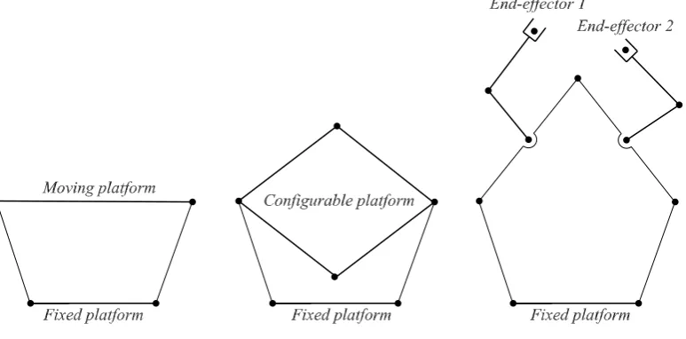
Figure1shows how the concepts of configurable platform and multiple end-effectors can improve 48
considerably the capacity of a simple closed kinematic chain yielding, in this case, a hybrid robot 49
manipulator (HRM), e.g., the end-effectors of the HRM would work together as two cooperating 50
manipulators in addition to the typical operations of serial and parallel manipulators. The idea is 51
simple but effective. Firstly, the four-bar mechanism is considered as a parallel manipulator where the 52
coupler link is chosen as the moving platform. Secondly, the moving platform is transformed into a 53
configurable platform formed with four articulated bars. Finally, two of the articulated links of the 54
configurable platform are removed, a practical decision, and one 2R open kinematic chain playing the 55
role of end-effector is attached to each one of the remaining links of the configurable platform. 56
Figure 1.Transition of a closed kinematic chain into a hybrid robot manipulator
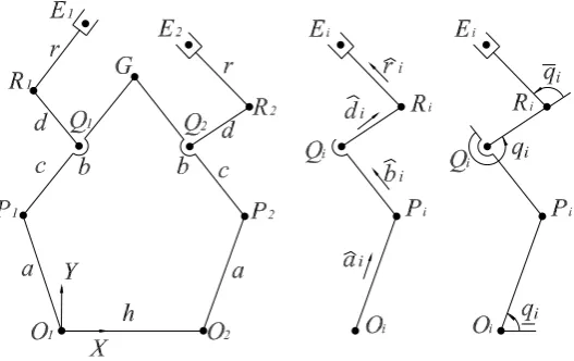
Hence, the proposed robot manipulator, right planar mechanism of Fig. 2, consists of two 57
end-effectors sharing a five-bar planar mechanism. The five-bar mechanism is a planar parallel 58
mechanism which owing its two degrees of freedom is used for positioning a point on a region of the 59
workspace. The five bars are serially connected by means of revolute joints where conveniently the 60
two revolute joints mounted on the base link are actuated. 61
In order to explain the geometry of the HRM let us consider thatXYis a reference frame attached 62
to the base link whose origin is located at pointO1, see Fig.2. Afterwards, let us consider thath 63
denotes the length of the base link while the lengths of the lower and upper links of the legs of the 5R 64
mechanism are denoted, respectively, byaandb. The orientation of the lower links is controlled by 65
means of the lower generalized coordinatesq
Figure 2.Geometry scheme of the hybrid robot manipulator
oooi. Unless otherwise, in the rest of the paperi=1, 2. The end of the lower links are denoted by points 67
Pilocated by vectorspppi. The output point of the 5R mechanism is the pointGwhich is located by vector 68
gggand of course also is the common point of the two legs of the 5R mechanism. Theith 2R serial chain 69
is connected to the 5R mechanism through a revolute joint denoted by pointQi, located by vectorqqqi, in 70
whichcdenotes the distance between pointsPiandQi. The arm and forearm of theith end effector are 71
denoted by the lengthsdandrand are articulated by means of a revolute joint characterized by point 72
Ri, located by vectorrrri. Naturally, the revolute joints of the end-effectors are actuated according to 73
the middle and upper generalized coordinatesqiand ¯qi. Thus the set of generalized coordinates are 74
notated as{qi,qi, ¯qi}. Finally, the positions of the end-effectors are denoted by pointsEi, located by 75
vectorseeei. With the purpose to arrive at pointEi, beginning from pointOi, let us consider four unit 76
vectors: i) ˆaaaiexpresses a unit vector pointed fromOitoPi, ii) ˆbbbidenotes a unit vector directed fromPi 77
toQi, iii) ˆdddistands for a unit vector pointed fromQitoRiand, iv) ˆrrriis a unit vector specified fromRi 78
toEi. 79
3. Displacement analysis 80
In this section the finite kinematics of the HRM manipulator is presented. 81
3.1. Displacement Analysis of the 5R Mechanism 82
3.1.1. Forward Displacement Analysis of the 5R Mechanism 83
The forward displacement analysis consists of finding the coordinates of the output pointG= (XG,YG)given the lower generalized coordinatesqi. SinceGis described by the vectorgggthen the analysis may be solved based on the following two closure equations
(ggg−pppi)·(ggg−pppi) =b2 (1) in whichpppi=oooi+aˆaaaiwhere ˆaaai =cosqiˆiii+sinqiˆjjj. Meanwhile the dot(·)denotes the inner product of three-dimensional vector algebra. From expressions (1) one obtains two quadratic equations in the unknown coordinatesXGandYG which may be reduced after a few computations into two simple equations as follows
(1+K21)X2G+2(K1K2−acosq1−K1asinq1)XG+a2−b2+K22−2K2asinq1=0,YG=K1XG+K2 (2) where the coefficientsK1andK2are given by
K1= (acosq1−acosq2−h)/a(sinq2−sinq1) 85
K2= (hacosq2+h2/2)/a(sinq2−sinq1) 86
As it was expected, given the parameters of the 5R mechanism and the lower generalized coordinates 87
q1andq2, the output pointGcan reach at most two positions. 88
3.1.2. Inverse Displacement Analysis of the 5R Mechanism 89
The inverse displacement analysis of the 5R mechanism consists of finding their configurations given the coordinates of pointG, e.g., it is required to compute the lower generalized coordinatesqi given the coordinates of pointG. To this end from Eq. (1) an expression of the form
Aisin(qi) +Bicos(qi) =Ci (3) is easily derived in which the coefficients are given by
90
Ai=2aYG, 91
Bi =2aXG−2δiahwhereδ1=0,δ2=1, 92
Ci=X2G+YG2+a2−b2+δih2 93
Equation (3) yields a quadratic equation in the unknown sinqias follows
(A2i +B2i)sin2qi−2AiCisinqi+C2i −Bi2=0 (4) Therefore there are four possible solutions for the inverse displacement analysis of the 5R mechanism. 94
3.2. Displacement Analysis of the Open Kinematic Chains 95
In order to approach the displacement analysis of the two open kinematic chains let us consider that the position vectoreeeiofEimay be obtained as
eeei =oooi+aˆaaai+cbbbˆi+ddddˆi+rˆrrri (5) Therein, the unit vectors ˆdddiand ˆrrrimay be obtained as ˆdddi=Rqibbbˆiand ˆrrri=Rqi¯dddˆiwhere Rqiand Rqi¯ are 96
the usual rotation matrices built according to the middle and upper generalized coordinatesqiand ¯qi, 97
respectively. Meanwhile, it is evident that ˆbbbi= (ggg−pppi)/b. 98
3.2.1. Forward Displacement Analysis of the Open Kinematic Chains 99
This analysis comprises the computation of the coordinates of pointsEifor a set of generalized 100
coordinatesqi,qiand ¯qi. Once the forward displacement analysis of the 5R mechanism is solved, see 101
subsection3.1.1, the coordinates ofEiare obtained by a direct application of Eq. (5). Hence, each point 102
Eican reach at most two locations. 103
3.2.2. Inverse Displacement Analysis of the Open Kinematic Chains 104
This analysis deals with the computation of the generalized coordinates of the HRM given the coordinates of pointsEi. The possibilities of this analysis are immense due to the inclusion of extra generalized coordinates. For example assuming values for the lower revolute joints, then the coordinates of pointsQi, which are located by vectorsqqqi, may be resolved taking into account that qqqi =oooi+cbbbˆi. Afterwards, with the purpose to compute the generalized coordinatesQi andRi the following closure equations would be considered for each open chain
(eeeˆi−rrri)·(eeeˆi−rrri) =e2i, (rrrˆi−oooi−cbbbˆi)·(rrrˆi−oooi−cbbbˆi) =r2 (6) Following the method of the displacement analysis realized for the 5R mechanism, the position 105
vectorsrrriare determined solving Eqs. (6), and the computation of the generalized coordinatesqiand 106
¯
4. Instantaneous Kinematics 108
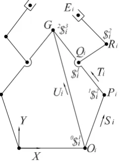
In this section the velocity and acceleration analyses of the HRM are addressed by means of 109
the theory of screws. The screws representing the revolute joints and reciprocal lines of the robot 110
manipulator are shown in Fig.3. For details of this section the reader is referred to Gallardo-Alvarado 111
[8]. 112
Figure 3.The screws of the hybrid robot manipulator
Let us consider thatmis a rigid body in motion with respect to another body or reference frame labeled 0. Furthermore, let us consider that0ωωωmis the angular velocity vector ofmas measured from the reference frame 0 whilevvv∗is the linear velocity vector of an arbitrary point(∗)ofm. The vectors 0
ω ω
ωmandvvv∗form an inseparable entity named the velocity state ofmwith respect to 0, notated as 0VVVm. In fact, the velocity state of bodymis defined as a six-dimensional vector0VVVmcreated with two concatenated vectors namely the primal and dual parts of the velocity state notated asp(0VVVm) andd(0VVVm), respectively. The first one is the vector0ωωωmwhile the second one is the vectorvvv∗, i.e., 0VVVm ≡ (p(0VVVm),d(0VVVm)) = (0
ω ω
ωm,vvv∗). The confirmation of the equivalence of the velocity state of rigid body as a twist about a screw is one of the most relevant contributions of the theory of screws to the study of the kinematics of rigid body, specially in the field of robot kinematics, e.g., assuming that mis the end effector of an open kinematic chain while 0 is the base link then the velocity state ofmas measured from 0 may be expressed as a linear combination of the infinitesimal screws representing the kinematic pairs of the open chain as follows
0VVVm =
0ω10$1O+1ω21$2O+. . .+m−2ωm−1m−2$m−1O+m−1ωmm−1$mO (7) wherek−1ωkis the joint rate between the adjacent bodiesk−1 andkwhileOis the reference point for computing the Plücker coordinates of the infinitesimal screws, also known as the reference pole. If the reference pole(O)is the point(∗)then0VVVm
∗ =0VVVm. Otherwise, according to the theory of helicoidal vector fields we have
0VVVm
∗ =
"
p(0VVVm)
d(0VVVm) +p(0VVVm)×rrr∗/O
#
(8)
whererrr∗/Ois the position vector of∗with respect toO. 113
On the other hand, the reduced acceleration state, or accelerator for brevity, of rigid bodym as observed from body 0 is defined as a six-dimensional vector0AAAm built with two concatenated vectors namely the primal and dual parts of the accelerator. The primal part corresponds to the angular acceleration vector0αααm, i.e. 0αααm = dtd0ωωωm, while the dual part is a composed vector given byaaa∗−0
ω
accelerator is defined as0AAAm≡(p(0AAAm),d(0AAAm)) = (0αααm,aaa∗−0ωωωm×vvv∗). Furthermore, in an open serial chain the accelerator may be written in screw form as follows
0AAAm=
0α10$1O+1α21$2O+. . .+m−2αm−1m−2$m−1O+m−1αmm−1$mO+0LLLm (9) wherek−1αk= dt kd −1ωk. Meanwhile,0LLLmis the Lie screw of acceleration which is given by
114
0LLLm=h
0ω10$1O 1ω21$2O+. . .+m−2ωm−1m−2$m−1O+m−1ωmm−1$mO
i
+h1ω21$2O 2ω32$3O+. . .+m−2ωm−1m−2$m−1O+m−1ωmm−1$mO
i
+. . .+hm−2ωm−1 m−2$m−1O+m−1ωmm−1$mO
i
(10)
4.1. Instantaneous Kinematics of the 5R Mechanism 115
Let us consider that0VVVGG = (ωωω,vvvG)is the velocity state ofG as observed from the base link, where point G plays the role of reference pole. It is evident that due to the planar nature of the robot manipulator at hand some terms of the velocity state vanish, i.e., 0VVVGG = (ωωω,vvvG) =
h
0 0 ωZ vGX vGY 0
iT
. On the other hand, the velocity state0VVVGG may be written in screw form as follows
0VVVG
G=0ωi10$1i +1ω2i1$2i +2ω3i2$3i (11)
where0ωi1=q˙
iis theith lower generalized velocity. 116
In order to obtain the linear input-output equation of velocity of the 5R mechanism let us consider thatTTTiis a line in Plücker coordinates directed fromPitoG, e.g. TTTi = (bbbi, 000)advised thatGis the reference pole. The application of the Klein form of the lineTTTito both sides of expression (11) with the reduction of terms leads to
{TTTi;0VVVGG}=q˙i{TTTi;0$1i} (12) Hence, after a few computations the linear input-output equation of velocity of the 5R mechanism results in
JT
"
vGX vGY
#
=J Qv (13)
where 117
J=hbbb1ˆ bbb2ˆ iis the direct Jacobian matrix of the 5R mechanism, 118
J=diagh{TTT1;0$11} {TTT2;0$12}iis the inverse Jacobian matrix of the 5R mechanism, and 119
Qv=
h
˙ q
1 q˙2
iT
is the first-order driver matrix of the 5R mechanism. 120
In order to compute the passive joint velocity rates1ωi2and2ω3i, a necessary step for approaching the acceleration analysis, let us consider two lines in Plücker coordinates for each leg of the 5R mechanism: i)UUUiis a line pointed fromOitoG, i.e.UUUi= (uuuˆi, 000)where ˆuuui = (ggg−oooi)/|ggg−oooi|, ii)SSSi is a line pointed fromOitoPi, i.e.SSSi = (aaaˆi, ˆaaai×rrrG/Oi). Thus by taking advantage of the concept of
reciprocal screw it follows that
1ωi2={UUUi;0VVVGG}/{UUUi;1$2i}, 2ω3i ={SSSi;0VVVGG}/{SSSi;2$3i} (14) Finally, once the joint velocity rates1ωi2 and2ωi3are computed, the angular velocity vector ωωω is 121
obtained as the primal part of0VVVGGby resorting to Eqs. (11), (17) and (14). 122
i.e.,0AAAGG = (ααα,aaaG−ωωω×vvvG) =
h
0 0 αZ aGX+ωZvGY aGY−wZvGX 0
iT
. Furthermore, the
accelerator0AAAGGmay be written in screw form as follows 0AAAG
G =0αi10$1i +1αi21$i2+2αi32$i3+0LLLGiG (15) where0αi1 = q¨
i is the ith lower generalized acceleration. Meanwhile, 0LLLGi
G is theith Lie screw of acceleration which is calculated as follows
0LLLGi G =
h
0ωi10$1i 1ωi21$2i +2ωi32$3i i
+h1ω2i1$i2 2ωi32$3i i
(16)
where the brackets,[∗ ∗], denote the Lie product or outer product of the Lie algebrase(3)of the 123
Euclidean groupSE(3). 124
Following the trend of the velocity analysis, the linear input-output equation of acceleration of 125
the 5R mechanism results in 126
JT
"
aGX+ωZvGY aGY−ωZvGX
#
=J Qa+
"
{TTT1;LLLG1} {TTT2;LLLG2}
#
(17)
where Qa =
h
¨
q1 q¨2iT is the second-order driver matrix of the 5R mechanism. Furthermore, the 127
passive joint acceleration rates are given by 128
1αi2={UUUi;0AAAGG−0LLLGiG}/{UUUi;1$2i}, 2ωi3={SSSi;0AAAGG−0LLLGiG}/{SSSi;2$3i} (18) 4.2. Instantaneous Kinematics of the Open Chains
129
Once the passive joint velocity rate1ωi2was computed, see Eq. (14), the velocity state of theith end-effector may be determined as follows
0VVVEi
G =q˙i0$1i +1ω2i1$2i +q˙i$1i +q˙¯i$2i (19) Furthermore, according to the theory of helicoidal vector fields, the velocity state of theith end-effector considering pointEias the reference pole is given by
0VVVEi Ei=
" ωωωEi
vvvEi
#
=
"
p(0VVVEiG) d(0VVVEi
G) +p(0VVVEiG)×rrrEi/G
#
(20)
whererrrEi/Gis the position vector ofEiwith respect toG. Meanwhile,ωωωEiis the angular velocity vector 130
of theith end-effector whereasvvvEi is the velocity of pointEi. It is worth to note that according to 131
Eq. (19) there is a unique solution for solving the forward velocity analysis given the joint velocity rates 132
˙ q
i, ˙qiand ˙¯qiwhereas for the solution of the inverse velocity analysis there is an infinite of possibilities, 133
e.g., given the velocity state0VVVEiEione can freely choose arbitrary lower generalized speeds ˙q1and ˙q2 134
and then the computation of the required values of ˙qiand ˙¯qiis straightforward by resorting to Eq. (19). 135
With the purpose to approach the acceleration analysis let us consider that the accelerator of the ith end-effector may be written in screw form as follows
0AAAEi
G =q¨i0$1i +1αi21$2i +q¨i$1i +q¨¯i$2i +0LLLEiG (21) where theith Lie screw of acceleration0LLLEiG is computed as
0LLLEi G =
h
˙
qi0$1i 1ω2i1$2i +q˙i$1i +q¨¯i$2i
i
+h1ω2i1$2i q˙i$1i +q˙¯i$2i
i
+hq˙i$1i q˙¯i$2i
i
As it was expected, the solution of the forward acceleration analysis of the HRM is unique while 136
for the inverse acceleration analysis we have an infinite of solutions, a virtue of the redundancy of 137
HRM. On the other hand, by resorting to the theory of helicoidal vector fields it follows that the 138
reduced acceleration state of theith end-effector takingEias the reference pole may obtained as 139
0AAAEi Ei=
" α ααEi aaaEi−αααEi×vvvEi
#
=
"
p(0AAAEiG)
d(0AAAGEi) +p(0AAAEiG)×rrrEi/G
#
(23)
whereαααEiis the angular acceleration vector of theith end-effector whileaaaEiis the linear acceleration 140
vector of pointEi. 141
5. Numerical Example 142
In order to show the application of the method of kinematic analysis, in this section a case study 143
is provided. In that concern it is interesting to take into account that Huang [9] applied a parametric 144
variation method with the purpose to optimize the dimensions of the 5R mechanism according to the 145
solution of a multi-variable non-linear system generated with the objective to enlarge the workspace 146
and also to alleviate singularities. The optimal parameters of that research for the 5R mechanism was 147
proposed asa=1.9m,b= 2.1m,h= 1.407m. In the contribution the remaining parameters of the 148
HRM manipulators are chosen asc=b/2=1.05m,d=0.75m,r=0.5m. There is nothing special in 149
these last parameters. 150
The first part of the example deals with the forward displacement analysis. With this hope, assume 151
that the generalized coordinates are given byq
1 = 125
o,q
1 = 55o, ¯q1 = 280o,q2 = 50o,q2 = 245o,
152 ¯
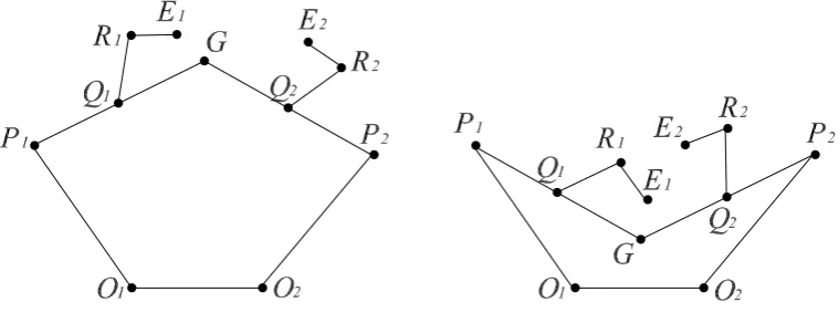
q2=110o. After a few computations, the application of the method explained in section3.2yields two 153
possible configurations of the HRM which are illustrated in Fig.4. 154
Figure 4.Case study. Available configurations of the hybrid robot manipulator
The next part of the exercise is devoted to the numerical solution of the instantaneous kinematics 155
of the HRM. To this end let us consider that upon the reference configuration, left pose of Fig.4, the 156
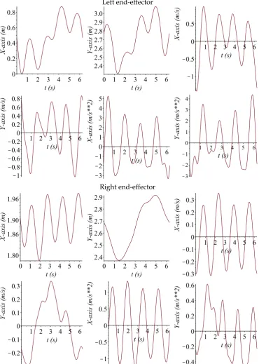
generalized coordinates are commanded to follow periodical functions given by 157
q1=0.15 sin(t),q1=0.25[sin(t) +sin(4t) +sin(2t)cos(t)], ¯q1=0.25 sin(t)cos(t), q2=−0.1 sin(t),q2=0.1[sin(4t)−sin(t)], ¯q2=−0.1 sin(t)
where the timetis given in the interval 0 ≤t ≤2π. Said otherwise, the period of the generalized 158
coordinates is 2π. The temporal behavior of the kinematics of the end-effectors by applying the 159
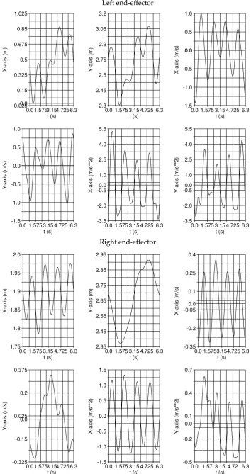
Furthermore, the numerical results shown in Fig.5are compared with results obtained using 161
another approach such as special software like ADAMS,TMthe corresponding plots are given in Fig.6. 162
Finally, it is worth to note that the results obtained by applying the theory of screws are in excellent 163
agreement with those generated with ADAMS.TM 164
6. Conclusions 165
In this work the kinematics of a hybrid robot manipulator composed of two 2R open kinematic 166
chains sharing a five-bar planar mechanism is approached by means of the theory of screws. The 167
displacement analysis of the HRM is easy to follow owing the fact that closed-form solutions are 168
obtained based on closure equations that lead us simple quadratic equations. After, the instantaneous 169
kinematics of the HRM is carried out by solving firstly the velocity and acceleration analyses of the 170
five-bar planar mechanism. The input-output equations of velocity and acceleration of the five-bar 171
mechanism are systematically obtained by resorting to reciprocal-screw theory. Finally, the velocity 172
and acceleration analyses of the end-effectors are performed by considering that their revolute joints 173
are actuated. A case study is included with the purpose to exemplify the method of kinematic analysis. 174
Furthermore, the numerical results of the instantaneous kinematics of the case study obtained by 175
means of the theory of screws were verified with the aid of commercially available software like 176
ADAMS.TM 177
Acknowledgment 178
The first author acknowledge with thanks the support of the National Council of Science and 179
Technology of Mexico (CONACYT) through National Network of Researchers (SNI) fellowship. Grant 180
number 7903. 181
Author Contributions 182
The displacement analysis of the hybrid robot manipulator was carried out by Ramon 183
Rodriguez-Castro and Luciano Perez-Gonzalez. Jaime Gallardo-Alvarado realized the velocity and 184
acceleration analyses of the HRM as well as the solution of the numerical examples. Carlos R. 185
Aguilar-Najera made the translation of the mathematical framework developed for the kinematics of 186
the HRM into computer codes. Alvaro Sanchez-Rodriguez modeled the HRM in the special software 187
of simulation ADAMS.TMJaime Gallardo-Alvarado is the first author of the contribution. 188
Conflicts of Interest 189
The authors declare no conflict of interest. 190
191
1. Hoevenaars, A.G.L.; Gosselin, C.; Lambert, P.; Herder, J.L. A systematic approach for the Jacobian analysis of
192
parallel manipulators with two end-effectors.Mech. Mach. Theory2017,109, 171-194.
193
2. Balli, S.S.; Chand, S. Synthesis of a five-bar mechanism with variable topology for motion between extreme
194
positions (SYNFBVTM).Mech. Mach. Theory2001,36, 1147-1156.
195
3. Liu, X.-J.; Wang, J.; Pritschow, G. Kinematics, singularity and workspace of planar 5R symmetrical parallel
196
mechanisms,Mech. Mech. Theory2006, 41, 145-169.
197
4. Joubair, A.; Slamani, M.; Bonev, I.A. Kinematic calibration of a five-bar planar parallel robot using all working
198
modes.Mech. Mach. Theory2013, 29, 15-25.
199
5. Nafees, K.; Mohammad, A. Synthesis of a planar five-bar mechanism consisting of two binary links having
200
two offset tracing points for motion between two extreme positions.ASME J. Mech. Robot.2016,8, Paper No:
201
JMR-15-1302.
202
6. Six, D.; Briot, S.; Chriette, A.; Martinet, P. A controller avoiding dynamic model degeneracy of parallel robots
203
during singularity crossing.ASME J. Mech. Robot.2017,9, Paper No: JMR-17-1046.
7. Briot, S.; Goldsztejn, A. Topology optimization of industrial robots: Application to a five-bar mechanism.Mech.
205
Mach. theory2018,120, 30-56.
206
8. Gallardo-Alvarado, J.Kinematic Analysis of Parallel Manipulators by Algebraic Screw Theory. Springer International
207
Publishing,2016.
208
9. Huang, M.Z. Design of a planar parallel robot for optimal workspace and dexterity.Int. J. Adv. Robot. Sys.2011,
209
8, 176-183.
Left end-effector
Right end-effector
Left end-effector 6.3 4.725 3.15 1.575 0.0 0.0 1.025 0.85 0.675 0.5 0.325 0.15 -0.025 t (s) X-axis (m) 6.3 4.725 3.15 1.575 0.0 3.2 3.05 2.9 2.75 2.6 2.45 2.3 t (s) Y-axis (m) 6.3 4.725 3.15 1.575 0.0 0.0 1.0 0.5 0.0 -0.5 -1.0 -1.5 t (s) X-axis (m/s) 6.3 4.725 3.15 1.575 0.0 0.0 1.0 0.5 0.0 -0.5 -1.0 -1.5 t (s) Y-axis (m/s) 6.3 4.725 3.15 1.575 0.0 0.0 5.5 4.0 2.5 1.0 -0.5 -2.0 -3.5 t (s) X-axis (m/s**2) 6.3 4.725 3.15 1.575 0.0 0.0 5.5 4.0 2.5 1.0 -0.5 -2.0 -3.5 t (s) Y-axis (m/s**2) Right end-effector 6.3 4.725 3.15 1.575 0.0 2.0 1.95 1.9 1.85 1.8 1.75 t (s) X-axis (m) 6.3 4.725 3.15 1.575 0.0 2.95 2.85 2.75 2.65 2.55 2.45 2.35 t (s) Y-axis (m) 6.3 4.725 3.15 1.575 0.0 0.0 0.4 0.25 0.1 -0.05 -0.2 -0.35 t (s) X-axis (m/s) 6.3 4.725 3.15 1.575 0.0 0.0 0.375 0.2 0.025 -0.15 -0.325 t (s) Y-axis (m/s) 6.3 4.725 3.15 1.575 0.0 0.0 1.5 1.0 0.5 0.0 -0.5 -1.0 -1.5 t (s) X-axis (m/s**2) 6.3 4.72 3.15 1.57 0.0 0.0 0.7 0.4 0.1 -0.2 -0.5 t (s) Y-axis (m/s**2)