http://www.sciencepublishinggroup.com/j/earth doi: 10.11648/j.earth.20190806.14
ISSN: 2328-5974 (Print); ISSN: 2328-5982 (Online)
Optimization of Soil Sampling Design Based on Road
Networks – A Simulated Annealing/Neural Network
Algorithm
Rong Chen
1, Shishi Liu
1, Yufei Yang
1, Wei Huang
1, *, Zongwei Han
2, Peihong Fu
11
College of Resource and Environment, Huazhong Agricultural University, Wuhan, China 2Department of Tourism and Geography, Tongren University, Tongren, China
Email address:
*
Corresponding author
To cite this article:
Rong Chen, Shishi Liu, Yufei Yang, Wei Huang, Zongwei Han, Peihong Fu. Optimization of Soil Sampling Design Based on Road Networks – A Simulated Annealing/Neural Network Algorithm. Earth Sciences. Vol. 8, No. 6, 2019, pp. 335-345. doi: 10.11648/j.earth.20190806.14
Received: September 27, 2019; Accepted: November 6, 2019; Published: November 22, 2019
Abstract:
In this study, the spatial distribution pattern of the roads, historical samples, digital elevation data, and other available resources were incorporated into the design of a soil-sampling scheme to predict the soil organic matter (SOM) of the northern region of Zhongxiang City, Hubei Province, and simulated annealing (SA) was applied to optimize the sampling design. The sampling points determined after optimization were used to establish a multivariate linear regression model to adequately reproduce the intrinsic link between topographic factors and the SOM at 13 different sampling scales in areas nearby the existing roadways in the study area. The topographic factors included slope, plane curvature, profile curvature, topographic wetness index (TWI), stream power index (SPI), and sediment transport index (STI). A multilayer perceptron (MLP) model was also constructed. Comparison of the accuracy of the multivariate linear regression and MLP models demonstrated the feasibility of an optimized soil sampling design based on the road network. With the optimized sampling design, accurate soil-landscape information can be obtained, and its precision is greater than that of the original sampling scheme before optimization. The optimized sampling design obtained reduces sampling costs, increases sampling efficiency, and provides an effective method for obtaining the spatial distribution pattern of organic matter in soils.Keywords:
Soil-landscape Model, Simulated Annealing (SA), Multilayer Perceptron (MLP), Sampling Design Optimization1. Introduction
The soil sampling design with specific spatial layouts aims to obtain accurate soil attributes over a broad area. It plays an important role in the arable land fertility assessment, precision agriculture, and digital soil mapping. Collecting soil samples in the field requires tremendous work and resources, and it is therefore critical to establish an optimal sampling distribution and the number of total samples. Conventional soil sampling methods can be divided into three broad categories: classical sampling that involves collecting a large number of samples within a specific distribution pattern [1], spatial sampling that uses the spatial autocorrelation of geographic attributes [2], and purposive sampling, which is a non-random method that depends on prior knowledge and data mining technology [3].
Soil sampling design begins from the premise of an appropriate sampling scale, and seeks to ensure that the sample set presents an adequate representation of the entire area. Typically, sampling design can be optimized with expert knowledge approaches, geostatistics, or approaches based on representativeness of sample [4-6]. These methods, however, suffer from limitations such as a dependence on empirical knowledge, second-order stationary assumptions, and quasi-intrinsic assumptions [7].
via X-ray diffraction [8]. The design of the sampling scheme can also be optimized by developing a spatial map of soil properties (e.g. soil salinity, clay content and pH) based on the soil conductivity derived from electromagnetic induction
[9-10]. Moreover, the representativeness of spatial
distributions of soil salinity has been improved using predictive models based on remote sensing data to reduce the number of on-site samples [11]. Models that account for the effects of spatial differences in soils have been employed to assist the sampling design. For example, to balance the accuracy and cost of soil sampling, mathematical diffusion models have been used to determine optimal sampling densities [12]. Analysis of the spatial layout of soil properties has also employed soil environment reasoning models to improve the predicative precision of a limited number of sampling points [13]. Such considerations of the spatial distributions of soil attributes, including cofactors, seek to ensure that the layout of the fewest possible number of sampling points represent the overall environment. In this manner, the optimization of the sampling design is achieved. Topographic features and road networks also have spatial distribution patterns, and can be used as cofactors in the soil sampling design.
It is of significant interest to note that road networks ease the field soil sampling work over large areas. Road networks are characterized by a specific structure and spatial density that have a bearing on the usefulness of the road network as a cofactor in soil sampling design. Moreover, with the continued development of urban-rural integration, the density and spatial layout of road networks are expected to be gradually stabilizes [14]. For field soil sample collection on a countywide scale, the location of the sampling points and the sampling sequence can be roughly determined according to the road layout. However, researches that optimize the soil sampling strategies with the spatial distribution of networks are quite limited.
To acquire the soil-landscape information inherent to the
typical soils of a region, several sampling points of high representativeness should be determined in the corresponding region based on the predictions of statistical models. The spatial distributions of soil properties show a continuous change [15]. For a sufficiently dense road network that covers the corresponding soil area, it can be expected that highly representative soil regions exist nearby the existing roadways. The sampling area can thus be established within a prescribed distance from roads, and the optimal layout of the sampling points can be arranged according to the distribution pattern of the road network. Since soil-landscape information remains stable over time, the knowledge and patterns of soil distribution contained in historical soil samples can be utilized. To optimize the soil sampling design and explore the overall soil properties, a soil organic matter (SOM) landscape model can be established to predict the SOM content. The SOM was chosen because SOM has a major impact on soil properties, although its fraction is minimal in soil.
In this study, the spatial distribution of the roads, historical samples, digital elevation data, and other available resources were incorporated into the design of a soil-sampling scheme. The simulated annealing (SA) was applied to optimize the sampling design. The sampling points determined after optimization were used to establish a multivariate linear regression model of the soil-landscape. Then, a multilayer perceptron (MLP) model was used to evaluate the predictive accuracy of the regression model, and this predictive precision was, in turn, used to assess the sampling design. The established MLP model was found to adequately reproduce the intrinsic link between topographic factors and the SOM, showing a high predictive precision. The MLP model can make efficient use of available knowledge, and provides strong generalization and nonlinear mapping abilities. Thus, the prediction results of this model can be used to test the SOM of sampling points after optimization.
2. Study Area and Methods
2.1. Study Area
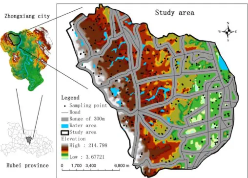
Figure 1. Location of the study area, road networks in the study area, and the spatial distribution of the historical sampling points. The shaded areas are 300-m
The study area is located in the northern region of Zhongxiang City, Hubei Province, China (31°21’–31°33’N, 112°13’–112°27’E), with an area of 244 km2. This location is in central Hubei Province, to the west of the upper Hanjiang River, as shown in Figure 1. The area is of mixed topography including hills, low mountains, and plains. The highest elevation is 215 m, and the elevation gradually decreases from west to east. The 319 historical sampling points shown in Figure 1 are distributed among different terrain and soil types, and were subjected to random sample collection in 2005–2006. The road network has a density of 0.78 km·km-2, which covers the entire study area with a rather uniform distribution.
2.2. Methods
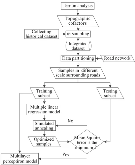
Figure 2. Flowchart of the proposed method.
The development and distribution of soil within the overall landscape result from interactions between numerous soil-forming factors [16]. The historical sampling data, regardless of the rationality of the spatial layout of the sampling points, provides soil-landscape knowledge specific to the region. The basic premise of the soil sampling design method proposed in the present study is as follows (Figure 2). Digital elevation model is used in the terrain analysis to obtain topographic cofactors. Widely distributed historical samples are collected and re-sampled with the topographic cofactors. The integrated dataset is partitioned based on road network. The samples from both sides of the scale’s roadways are employed. The soil-landscape relationship is established using multiple linear regressions of the topographic cofactors. Using the precision of the soil-landscape model as the objective function, an SA algorithm is subsequently applied to optimize
the sample set of the spatial layout iteratively until the error of the soil-landscape model is minimized. The initial and optimized data sets are then used to establish the MLP model, and the test data set is used to compare the precision of the model before and after sampling optimization to evaluate the performance of the optimization.
2.2.1. Selection and Acquisition of Topographic Cofactors
The significance of different topographic factors varies among landscapes. We used previous soil-landscape studies [17-18] to select commonly used topographic factors that have major impacts on the actual soil environment. The topographic cofactors chosen to characterize the soil distribution in the study area include elevation, slope, plane curvature, profile curvature [19], topographic wetness index (TWI) [20], stream power index (SPI) [21], and sediment transport index (STI) [22]. Digital elevation model (DEM) raster data with a 30 m resolution were obtained from the international scientific data mirror site maintained by the Computer Network Information Center of the Chinese Academy of Sciences (http://datamirror.csdb.cn), and were used to calculate the topographic factors. To provide smooth and continuous data, the above factors were calculated at a 10 m resolution. The topographic factors at the historical sampling points were extracted to ensure that the corresponding topographic factors appropriately represented the surrounding environment.
The soil sampling locations were based on the spatial distribution pattern of the roadways, and all sampling points were required to be at least 300 m away from all railways and roadways [23]. To explore the effects of the sampling scale on the precision of the final results, 13 sampling scales were established according to a 10-pixel increment (i.e., 100 m): 300–400, 300–500, ..., 300–1600 m. The sampling scale is the range over which samples can be obtained. The 300–1600 m scale covers the entire study area. At the same sample scale, overlapping regions between different roads were combined. At each sampling scale, the historical samples served as the initial sample set, and these were randomly divided into the training data set and the test data set in a 2:1 ratio. The training dataset therefore accounted for 2/3 of the initial sample set, and was used to train the model. The remaining was the test dataset used to validate the model.
2.2.2. Establishment of the Soil-landscape Model
feed forward artificial neural network (ANN) types for non-linear function approximation task which learns the pattern of data by several layers with connected perceptrons [24-25]. In this study, the seven selected topographic factors were served as the input layer, and the output layer was the SOM content. In addition, the model incorporates two hidden layers. The conversion function employed by the software is its default hyperbolic tangent function, denoted as Tanh Axon, and the learning algorithm is the Momentum algorithm. The Step Size and Momentum Rate are both software defaults. The termination conditions were a maximum number of iterations of 105 and a threshold value of 10-4. Based on the input data, the optimal number of neurons in each hidden layer calculated by the software was 4. Since the weight corresponding to each factor is very important, the weights are continuously optimized during the neural network computation to achieve optimal prediction results. Due to the high uncertainty of the neural network method, the data were trained five times, and the weights obtained during each training session were saved in a separate file. The model corresponding to the weights with the most precise prediction results was selected to build the soil-landscape model.
2.2.3. Optimization of the Spatial Layout of the Sampling Points
The historical sample data were used to select highly representative sampling points to achieve the optimization of the spatial distribution of the sampling points. SA is a
stochastic computing technique, which employs a
combinatorial optimization algorithm that converges to a global optimum while effectively avoiding local optima [26]. The algorithm has no strict requirements for the initial state of the study object. Hence, the SA algorithm can be used to solve complex deterministic combinatorial optimization problems [27-28]. In the past study, SA optimization was used to predict the spatial distribution of soil properties with a minimum number of samples while maintaining a predictive precision that was no smaller than that obtained using the original samples, thereby obtaining an optimal sample layout [27]. Another study used the average Kriging variance as the objective function in the SA algorithm [29]. In this case, the spatial layout of the samples was mainly assessed and optimized via two indicators, the main Kriging variance and the weighted Kriging variance, to obtain an optimum sampling design targeting different soil attributes. In the present study, the SA algorithm was applied, and the minimum
MSE of the SOM prediction was used as the criterion for optimization of the spatial layout of the soil sampling points to obtain the soil-landscape relationship with relatively high precision. The technique is therefore ideal for the present study because the determination of the optimal spatial layout of the sampling points is essentially a problem of combinatorial optimization between the sampling points. Each initial sample set was first optimized using the SA algorithm. The training data set was used to optimize the layout of the sampling points, and the test data set was used to validate the effectiveness of the optimized layout. A random subset of the training set was selected, and one of the remaining sampling points was randomly chosen to replace each point in the subset, one by one, until the sampling point in the subset most suitable for replacement was identified. This point was then replaced by the previously chosen point to form a new subset. Meanwhile, the multiple linear regression model of this data set was established, and the test data set was used to calculate the MSE, which is the objective function in the optimization process. During the iterative process described above, the MSE of each subset was determined based upon that subset’s multiple linear regression model, and the MSE values of all subsets were compared. The subset corresponding to the smallest MSE was then accepted. In this way, the optimal sample set with the minimum predictive error in each initial sample set was obtained. The remaining sampling points were redundant points under the principle of the minimum MSE.
2.2.4. Testing the Sample Layout Following Optimization
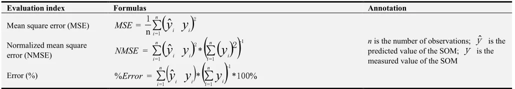
We quantitatively analyzed the extent to which the information contained in the original sample set was contained in the optimized data set, and determined the impact of optimization on the precision of the SOM prediction. The MLP models established using the optimized data and the multiple linear regression models established as described in Subsection 2.2.3 were used to predict the SOM content in the test sample set, and these values were compared with the actual measured values for error analysis. The evaluation indices used for assessing the models are listed in Table 1, the Akaike information criterion (AIC) was used to measure the complexity of the model and its goodness of fit, and the minimum description length (MDL) principle was used to measure the quality of the prediction of the decision attribute set by the condition attribute subset. Lower absolute values for the above two indicators indicate greater model precision.
Table 1. Overview of the evaluation indices used for assessing the models.
Evaluation index Formulas Annotation
Mean square error (MSE)
∑
(
)
1
2
1 n
i i i
y
y
MSE =ˆ
n =n is the number of observations;
y
ˆ
is the predicted value of the SOM;y
is the measured value of the SOMNormalized mean square
error (NMSE)
∑
1(
)
(
∑
1( )
)
2 n 2
i i
n
i i i
y
y
y
NMSE = -1 = * =ˆ
Error (%) % =
(
)
*( )
* %= -=
ˆ
∑
100∑
1 1 1 n i i ni
y
iy
iy
Evaluation index Formulas Annotation
Correlation coefficient (r)
(
) (
)
∑
−
∑
−
∑
−
−
= = = = n i i n i i n i ii
x
y
y
x
x
y
y
x
r 1 2 1 2 1 -1*
*n is the number of observations;
x
is the value of a particular topographic factor;x
is the mean value of the topographic factor;y
is the measured value of the SOM;y
is the mean value of the SOM Akaike information criterion(AIC) AIC = 2k-2ln( )L n is the number of observations; k is the
number of parameters; L is the likelihood function
Minimum description length
(MDL) MDL = 2kln( )n -ln( )L
1
3. Results and Discussion
3.1. Multiple Linear Regression Analysis of Topographic Factors Before and After SA Optimization
Table 2 shows the correlation between the topographic factors and the SOM.
Table 2. Pearson correlation coefficients between the soil organic matter (SOM) and the topographic factors in the study area.
SOM Elevation Slope Plan curvature Profile curvature Topographic Wetness index Stream power index Sediment Transport index
SOM 1
Elevation 0.47** 1
Slope 0.01 0.09 1
Plan curvature −0.09 −0.04 −0.04 1
Profile curvature 0.10 0.02 −0.02 −0.60** 1
Topographic
wetness index 0.00 −0.18** −0.16** 0.02 −0.07 1
Stream power
index 0.04 −0.10 0.20** 0.00 −0.06 0.82** 1
Sediment transport index
0.05 −0.02 0.14* 0.02 −0.05 0.30** 0.30** 1
**P<0.01; * P<0.05.
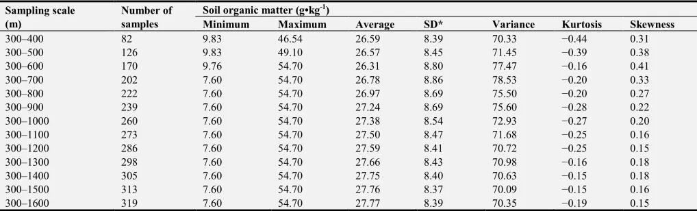
The number of sampling points and the SOM statistics at all sampling scales are listed in Table 3. The distribution patterns of the SOM are observed to be consistent at different sampling scales. The correlation coefficient (r) between the number of resampling points and the scale of the sampling area is 0.96, whereas the coefficient of determination of the linear
regression equation (R2) between the two is 0.91. Therefore the number of resampling points increases proportionally with the increasing scale of the sampling area and the ratio of the number of resampling points to the sampling scale is about 1.45 per square kilometer, which allows for comparison of the results obtained at different scales.
Table 3. Descriptive statistics of the soil organic matter in the study area with respect to the number of samples at each scale.
Sampling scale (m)
Number of samples
Soil organic matter (g•kg-1)
Minimum Maximum Average SD* Variance Kurtosis Skewness
300–400 82 9.83 46.54 26.59 8.39 70.33 −0.44 0.31
300–500 126 9.83 49.10 26.57 8.45 71.45 −0.39 0.38
300–600 170 9.76 54.70 26.31 8.80 77.47 −0.16 0.41
300–700 202 7.60 54.70 26.78 8.86 78.53 −0.20 0.33
300–800 222 7.60 54.70 26.97 8.69 75.50 −0.20 0.27
300–900 239 7.60 54.70 27.24 8.69 75.60 −0.28 0.22
300–1000 260 7.60 54.70 27.38 8.54 72.93 −0.27 0.20
300–1100 273 7.60 54.70 27.50 8.47 71.68 −0.25 0.16
300–1200 286 7.60 54.70 27.59 8.41 70.72 −0.25 0.15
300–1300 298 7.60 54.70 27.66 8.43 70.98 −0.16 0.18
300–1400 305 7.60 54.70 27.75 8.40 70.63 −0.15 0.18
300–1500 313 7.60 54.70 27.76 8.37 70.09 −0.15 0.16
300–1600 319 7.60 54.70 27.77 8.39 70.35 −0.19 0.15
*Standard deviation.
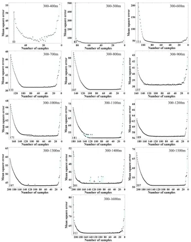
We used the SA algorithm to reduce the number of sampling points. In this process, each time one point is removed, and an MSE value of a multiple linear regression model was obtained. As illustrated in Figure 3, as the sampling scale increases, the
the MSE of the multiple linear regression model gradually decreases until reaching a fairly level value. However, after a continued reduction in the number of sampling points, the MSE of the model rises sharply, and graphs of the MSE vs. the number of sampling points exhibit a clear U shape at all sampling scales.
Results shown in Figure 3 indicates that when restricting sampling points to areas surrounding the roadways, the precision of the obtained soil-landscape model after sampling
design optimization is superior to that before optimization at a given sampling scale. For sampling points set nearby roadways, there exists an optimal spatial layout design for which the precision of the obtained SOM prediction model is relatively high. Because the number of sampling points increases as the sampling scale increases, the knowledge of the soil covered by the SOM prediction model is more comprehensive, and, thus, the predictive precision is improved.
Figure 3. MSE values of the SOM predictions versus the number of samples during the process of optimization at different sampling scales.
We examined the effects of sampling design optimization at different sampling scales by applying multiple linear regressions to the initial sample set and the sample set after SA optimization at each sampling scale. Table 4 compares the coefficients of these models. Different topographic factors characterize different aspects of the landscape, and, thus, the
nature and magnitude of the impact on the SOM differ among
different factors. Sample layout determines the
Table 4. Coefficients of multiple linear regression models for optimized and non-optimized sampling points at different sampling scales.
Sampling scale (m)
Constant Elevation Slope Plan curvature
Profile curvature
Topographic wetness index
Stream power index
Sediment transport index
a b a b a b a b a b a b a b a b
300–400 4.94 13.39 0.32 0.22 0.81 1.17 14.94 21.83 20.13 22.62 0.70 0.70 −0.52 −0.67 0.00 0.65 300–500 2.38 7.22 0.36 0.27 1.27 0.39 −3.14 −10.65 −7.81 18.94 0.58 0.90 −0.45 −0.34 0.14 −0.76 300–600 6.68 6.42 0.34 0.31 −0.03 0.97 −9.30 −0.86 −9.08 17.60 0.20 −0.47 0.10 0.93 −1.01 −1.57 300–700 10.51 7.39 0.32 0.28 −0.15 1.22 2.76 −15.38 7.00 −3.74 0.05 1.00 −0.06 −1.23 0.05 0.16 300–800 6.05 13.36 0.35 0.21 0.27 0.59 3.63 −10.56 3.18 2.10 0.06 0.39 0.04 −0.16 0.04 −1.31 300–900 9.45 8.02 0.28 0.34 0.07 −0.15 −3.94 −10.87 2.59 0.10 0.36 0.17 −0.06 0.01 −0.37 −1.10 300–1000 10.62 12.13 0.28 0.27 −0.02 −0.79 −1.37 −2.32 6.21 3.58 0.18 −0.07 0.12 −0.03 −0.07 1.32 300–1100 7.88 17.34 0.32 0.19 0.01 −0.44 1.22 −6.88 0.00 16.10 0.11 0.10 0.09 0.06 −0.03 −0.79 300–1200 9.26 11.72 0.31 0.21 −0.07 0.52 0.38 −3.46 7.00 4.99 0.11 1.41 0.10 −1.69 0.02 0.16 300–1300 7.62 15.08 0.32 0.22 −0.13 −0.78 −2.19 1.42 7.73 −2.37 0.11 0.16 0.13 −0.04 0.19 −0.25 300–1400 11.59 8.13 0.28 0.29 −0.43 0.31 −1.28 −7.77 7.25 −4.28 0.10 0.31 0.07 −0.13 0.02 −1.02 300–1500 10.49 16.83 0.30 0.19 −0.60 −0.17 −0.04 −4.90 9.40 −0.35 −0.16 −0.04 0.36 0.04 0.17 0.06 300–1600 11.60 12.79 0.27 0.26 −0.25 −0.37 1.41 −11.59 7.10 0.72 0.07 0.03 −0.05 0.26 0.40 −0.62
a: the value before optimizing; b: the value after optimizing.
3.2. Optimization Results of the Spatial Layout of the Sampling Points
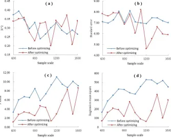
We compared the regression models obtained at different sampling scales before and after optimization by performing analysis of variance (ANOVA). Figures 4(a) and (b) show that when the sampling scale is 300–1100 m or is less than 300– 800 m, the coefficient of determination (R2) and standard error of the regression models after optimization of the sampling point layout are similar or less significant (i.e., lower R2 and higher standard error) than those before optimization. At all the other sampling scales, R2 and the standard error of the regression models after optimization are better than those before optimization. Figures 4(c) revealed that, before
optimization, the models at all sampling scales are statistically significant (P<0.05). After optimization, the models obtained at sampling scales 300–400 m and 300–1100 m are not statistically significant (P = 0.43 and P = 0.25, respectively), whereas, at sampling scales of 300–500 m, 300–800 m, and 300–1200 m, the models are all statistically significant (P = 0.02, P = 0.02, and P = 0.01, respectively). Figures 4(d) shows that, regression mean square of the regression models after optimization of the sampling point layout in different sample scale are less than those before optimization. Statistics shown in Figure 4 implies that sampling design optimization improves the precision of the regression model in most cases.
The predictive precisions and the numbers of samples of the regression models obtained at different scales before and after optimization are shown in Figure 5. Figure 5(a) demonstrates that, at the sampling scales 300–500 and 300–600 m, the precisions of the models before optimization are relatively low, as indicated by the rather large MSE values. At sampling scales greater than or equal to 300–700 m, the predictive precisions of the models before optimization significantly improve, with MSEs values smaller than 119.52 g·kg-1. The MSE of the multiple linear regression model obtained using the original sample set is large, indicating that the precision of the SOM prediction is relatively low. After SA optimization of
the sampling point layout, the MSEs of the models are no greater than 62.47 g·kg-1, and the predictive precision of the model after SA optimization is greater than that before optimization for all sampling scales. From Figure 5(b), the number of samples after SA optimization in each sampling scale is less than that before SA optimization. These results indicate that the SOM prediction of the model after optimization is closer to the actual measurements than the prediction of the model before optimization. Hence, SOM models with relatively high predictive precision can be obtained when limiting sampling points to areas surrounding the roadways after SA optimization.
Figure 5. Comparison of the predictive precision and the number of samples of the regression models at different sampling scales before and after optimization.
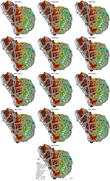
The comparisons of the spatial layouts of the sampling points before and after optimization at different sampling scales show that the sample points removed in the optimization are mainly located in low-elevation regions, valleys, and steep slopes (Figure 6). After optimization, the number of sampling points is substantially reduced, and this will notably decrease the workload and cost of the soil survey.
3.3. Precision of the SOM Prediction
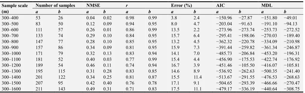
MLP models were separately established using the training data set and sample set after SA optimization, and the test data set was then used to quantitatively assess the precision of the SOM prediction by the sampling points before and after optimization. Table 5 lists the values for the evaluation indices given in Table 3 obtained for all MLP models established using the original sample set before and after optimization at the different sampling scales surrounding the roadways. The NMSE values are all less than or equal to 0.49, the values of r
are all greater than or equal to 0.71, the Error values are all less than or equal to 17.5%, and the absolute values of the AIC and MDL both first increase with the increasing sampling scale, and then begin to decrease at sampling scales greater than 300–1300 m. For MLP models established using optimized sampling points, the NMSE values, r values, and error values are all superior to those obtained before sampling optimization because points that have a negative effect on the predictive precision of the model are excluded during the optimization. Moreover, the absolute values of the AIC and MDL remain less than or equal to 336.19 and 308.75, respectively, which are smaller than those obtained before optimization for all sampling scales. In addition, these results indicate that the established MLP models can adequately reproduce the intrinsic link between the topographic factors and the SOM, and the predictive precision is relatively high. The prediction results of the MLP model can be used to evaluate the accuracy of the SOM prediction after sampling optimization.
Table 5. Precision of the multilayer perceptron model at different sampling scales.
Sample scale (m)
Number of samples NMSE r Error (%) AIC MDL
a b a b a b a b a b a b
300–400 53 26 0.04 0.02 0.98 0.99 3.8 2.4 −150.96 −27.87 −151.80 −49.01
300–500 83 50 0.12 0.09 0.94 0.95 8.0 4.7 −203.04 −91.63 −191.10 −94.13
300–600 111 57 0.26 0.01 0.86 0.99 13.5 2.2 −273.96 −273.74 −253.73 −272.52
300–700 133 74 0.29 0.10 0.84 0.95 15.7 6.4 −295.41 −198.06 −270.03 −189.40
300–800 147 77 0.28 0.10 0.85 0.95 13.2 4.5 −362.32 −220.78 −334.09 −210.98
300–900 157 86 0.34 0.09 0.81 0.95 15.9 7.3 −391.44 −259.82 −361.34 −246.87
300–1000 171 79 0.32 0.13 0.83 0.94 14.1 7.0 −485.73 −206.84 −453.20 −196.31
300–1100 181 52 0.40 0.03 0.77 0.99 15.4 4.4 −456.90 −175.53 −422.74 −176.92
300–1200 189 54 0.46 0.11 0.74 0.94 16.7 3.9 −451.46 −105.50 −416.07 −105.81
300–1300 195 115 0.31 0.28 0.83 0.85 14.6 8.9 −536.92 −262.63 −500.35 −241.40
300–1400 201 122 0.34 0.25 0.81 0.87 15.5 11.4 −513.67 −291.55 −476.53 −268.63
300–1500 207 95 0.42 0.40 0.76 0.78 17.1 9.1 −504.65 −293.39 −466.66 −270.47
300–1600 211 143 0.49 0.31 0.71 0.83 17.5 11.1 −479.17 −336.19 −440.64 −308.75
a: the value before optimizing; b: the value after optimizing.
For all MPL models, an increasing sampling scale introduces an increasing number of sampling points into the optimization process. Hence, the representativeness of the points selected from the historical samples must be improved. Both before and after optimization, the errors increase slowly with the increasing sampling scale. We used the MLP model with relatively high predictive precision to test the precision of the sampling points before and after optimization, and found that, after optimization, all indicators improved. This suggests that the sample set after optimization can represent the original sampling points, and be used to establish a soil-landscape model with a relatively high predictive precision.
4. Conclusion
This paper proposed a method for designing optimized soil sampling layouts in areas residing within a confined distance from existing roadways using the SA algorithm and historical sample data. The sampling scale nearby the roadways can be selected according to different precision requirements. The
achieve rational use of sampling resources while reducing the workload of the investigators.
Although the sampling design optimization method that targets areas surrounding roadways proposed in this study has yielded satisfactory results, several issues must be further examined. For example, the regression model selected to examine the relationship between the SOM and topographic features is a multiple linear regression model, and, for optimization of the sampling layout, the objective function used in the SA algorithm is the MSE. In addition, the parameters used to establish the MLP model for data testing (e.g., the number of hidden layers, training rules, and termination conditions) are set to the recommended default values provided by Neuro Solutions 6.31. The sensitivity of the SA algorithm to data quality also requires further exploration. In addition, experimental studies must be conducted to verify the applicability and efficiency of the proposed method for spatial sampling design targeting soil in other geological areas and in large-scale soil sampling.
Acknowledgements
This study was supported by the Natural Science Foundation of China (No. 41877001), National key research and development project (No.2017YFD0202000), and the Fundamental Research Funds for the Central Universities (2662019PY074). The author also sincerely thanks those who contributed to this article.
References
[1] Franzen, D. W. and Peck, T. R. (1995). Field Soil Sampling Density for Variable Rate Fertilization. Journal of Postdoctoral Affairs 8, 568-574.
[2] Cambardella, C. A., Moorman, T. B., Parkin, T. B., Karlen, D. L., Novak, J. M., Turco, R. F., et al (1994). Field-Scale Variability of Soil Properties in Central Iowa Soils. Soil Science Society of America Journal 58, 1501-1511.
[3] Shi, X., Zhu, A. X., Burt, J. E., Qi, F. and Simonson, D. (2004). A Case-based Reasoning Approach to Fuzzy Soil Mapping. Soil Science Society of America Journal 68, 885-894.
[4] Sakata, S., Ashida, F. and Zako, M. (2004). An efficient algorithm for Kriging approximation and optimization with large-scale sampling data. Computer Methods in Applied Mechanics and Engineering 193, 385-404.
[5] Thompson, A. N., Shaw, J. N., Mask, P. L., Touchton, J. T. and Rickman, D. (2004). Soil Sampling Techniques for Alabama, USA Grain Fields. Precision Agriculture 5, 345-358.
[6] An, Y., Yang, L., Zhu, A. X., Qin, C., and Shi, J. J. (2017). Identification of representative samples from existing samples for digital soil mapping. Geoderma 311, 109-119.
[7] Yang, L., Zhu, A. X., Qin C. Z., Li B. L., Pei T., Qiu W. L., et al (2010). A purposive sampling design method based on typical points and its application in soil mapping. Progress in Geography 29, 279-286. (in Chinese)
[8] Bertacchini, L., Durante, C., Marchetti, A., Sighinolfi, S.,
Silvestri, M., and Cocchi, M. (2012). Use of X-ray diffraction technique and chemometrics to aid soil sampling strategies in traceability studies. Talanta 98, 178-184.
[9] Huang, J., Lark, R. M., Robinson, D. A., Lebron, I., Keith, A. M., Rawlins, B., et al (2014). Scope to predict soil properties at within-field scale from small samples using proximally sensed γ-ray spectrometer and EM induction data. Geoderma 232–234, 69-80.
[10] Yao, R. j., Yang, J. s., Zhao, X. f., Chen, X. b., Han, J. j., Li, X. m., et al (2012). A New Soil Sampling Design in Coastal Saline Region Using EM38 and VQT Method. CLEAN – Soil, Air, Water 40, 972-979.
[11] Quan, Q. and Shen, B. (2012). A Soil Sampling Method Based on Field Measurements, Remote Sensing Images and Kriging Technique. Advanced Materials Research 383-390, 5350-5356.
[12] Wang, H., Yang, Q., Liu, Z. and Yang, C. (2006). Determining optimal density of grid soil-sampling points using computer simulation. Transactions of the Chinese Society of Agricultural Engineering 22, 145-148.
[13] Zhu, A. X., Hudson, B., Burt, J., Lubich, K. and Simonson, D. (2001). Soil Mapping Using GIS, Expert Knowledge, and Fuzzy Logic. Soil Science Society of America Journal 65, 1463-1473.
[14] Chan, S. H. Y., Donner, R. V. and Lämmer, S. (2011). Urban road networks — spatial networks with universal geometric features? The European Physical Journal B 84, 563-577.
[15] Yang, L., Zhu, A. X., Qin C. Z., Li B. L. and Pei T. (2011). A soil sampling method based on representativeness grade of sampling points. Acta Pedologica Sinica 48, 938-946. (in Chinese)
[16] Agbu, P. A., Ojanuga, A. G., and Olson, K. R. (1989). Soil-landscape relationships in the sokoto-rima Basin, Nigeria. Soil Science 148, 132-139.
[17] Gessler, P. E., Moore, I. D., McKenzie, N. J. and Ryan, P. J. (1995). Soil-landscape modelling and spatial prediction of soil attributes. International Journal of Geographical Information Systems 9, 421-432.
[18] Wang, J., Fu, B. and Qiu, Y. (2001). Soil nutrients in relation to land use and landscape position in the semi-arid small catchment on the loess plateau in China. Journal of arid environments 48, 537-550.
[19] Shary, P. A., Sharaya, L. S. and Mitusov, A. V. (2002). Fundamental quantitative methods of land surface analysis. Geoderma 107, 1-32.
[20] Tehrany, M. S., Pradhan, B., Mansor, S. and Ahmad, N. (2015). Flood susceptibility assessment using GIS-based support vector machine model with different kernel types. Catena 125, 91-101.
[21] Moore, I. D., Gessler, P. E., Nielsen, G. A. and Peterson, G. A. (1993). Soil Attribute Prediction Using Terrain Analysis. Soil Science Society of America Journal 57, 443-452.
[23] HJ/T166-2004, The technical specification for soil environmental monitoring. (in Chinese)
[24] Hamid, T. S., and Sahar, S. (2016). Statistical modeling approaches for pm10 prediction in urban areas; a review of 21st-century studies. Atmosphere 7, 15.
[25] Taewon Moon, Seojung Hong, Ha Young Choi, Dae Ho Jung, Se Hong Chang and Jung Eek Son (2019). Interpolation of greenhouse environment data using multilayer perceptron. Computers and Electronics in Agriculture 166, 105023.
[26] Kalivas, J. H. (1992). Optimization using variations of simulated annealing. Chemometrics and Intelligent Laboratory Systems 15, 1-12.
[27] Van Groenigen, J. W. and Stein, A. (1998). Constrained Optimization of Spatial Sampling using Continuous Simulated Annealing. Journal of environmental quality 27, 1078-1086.
[28] Zhang, S. J., Zhu A. X., Liu J. and Yang L. (2013). Soil sampling scheme based on simulated annealing method. Chinese Journal of Soil Science 44, 820-825. (in Chinese)