Article
1
Heterogeneous Deep Model Fusion for Automatic
2
Modulation Classification
3
Duona Zhang 1, Wenrui Ding 1, Baochang Zhang 1, Chunyu Xie 1, Chunhui Liu 1, Jungong Han 2
4
and Hongguang Li 1,*
5
1 School of Beihang University, Beijing 100083, P. R. China; [email protected]; [email protected];
6
[email protected]; [email protected]; [email protected]
7
2 School of Computing & Communications, Lancaster University, Lancaster LA1 4WA, U.K.;
8
9
* Correspondence: [email protected]; Tel.: +86-10-82317391
10
11
Abstract: Deep learning has recently attracted much attention due to its excellent performance in
12
processing audio, image, and video data. However, few studies are devoted to the field of
13
automatic modulation classification (AMC). It is one of the most well-known research topics in
14
communication signal recognition, which remains challenging for traditional methods due to the
15
complex disturbance from other sources. This paper proposes a heterogeneous deep model fusion
16
(HDMF) method to solve the problem in a unified framework. The contributions include: 1) The
17
convolutional neural network (CNN) and long short-term memory (LSTM) are combined by two
18
different ways without prior knowledge involved; 2) A large database, including eleven types of
19
single-carrier modulation signals with various noises as well as a fading channel, is collected with
20
various signal-to-noise ratios (SNRs) based on a real geographical environment; and 3)
21
Experimental results demonstrate that HDMF is super capable of copping with the AMC
22
problem, and achieves much better performance when compared with the independent network.
23
The source code and the database will be publically available.
24
Keywords: Deep learning; automatic modulation classification; classifier fusion; convolutional
25
neural network; long short-term memory
26
27
1. Introduction
28
Communication signal recognition is of great significance for several daily applications, such
29
as operator regulation, signal feature map generation, and user identification. One of the main
30
objectives of signal recognition is to detect the communication resources, which ensures the
31
reliability of communications. To achieve this objective, automatic modulation classification (AMC)
32
is indispensable because it can help users identify the modulation mode within a frequency band,
33
which benefits the communication reconfiguration and electromagnetic environment analysis.
34
AMC plays an essential role in obtaining digital baseband information from the signal when only
35
limited knowledge about the parameters is available. Such a technique is widely used in both
36
military and civilian applications, e.g., intelligent cognitive radio and anomaly detection [1]-[2],
37
which have attracted much attention from researchers in the past decades.
38
Basically, existing AMC algorithms can be divided into two main categories [3], namely,
39
likelihood-based (LB) methods and feature-based (FB) methods. LB methods require calculating the
40
likelihood function of received signals for all modulation modes and then make decisions in
41
accordance with maximum likelihood ratio test [3]. LB methods usually generate accurate
42
classification results but suffer from heavy computational cost. Alternatively, a traditional FB
43
method consists of two parts, namely, feature extraction and classifier, where classifier identifies
44
digital modulation modes in accordance with the effective feature vectors extracted from the signals.
45
As opposite to the LB methods, the FB methods are computationally light but may not be
46
theoretically optimal. To date, several FB methods have been validated effective on the AMC
47
problem. For instance, they successfully extract features from various time-domain waveforms,
48
such as cyclic spectrum [4], high-order cumulant [6], and wavelet coefficients. Afterwards, a
49
classifier is used for final classification based on features mentioned above. With the development
50
of learning algorithms, the performances have been improved, such as from the shallow neural
51
network [7] and decision tree to the support vector machine (SVM). Recently, deep learning is
52
widely applied to audio, image, and video processing, facilitating the applications such as face
53
recognition and voice discrimination [8]. However, a few works are done based on deep learning in
54
the field of communication.
55
Although researchers have developed various algorithms to implement AMC of digital signals,
56
these methods are suitable for simple communication equipment and struggle in the real-world
57
applications where more complicated equipment is in use, because: 1) they cannot handle complex
58
disturbance from other sources; 2)they usually separate feature extraction and classification process
59
so that the information loss is inevitable; and 3) those methods must use distributed receivers to
60
collect in-phase and quadrature signals, which costs additional storage space and bandwidth. In
61
this paper, we propose to realize AMC using the convolution neural networks (CNNs) [9], long
62
short-term memory (LSTM) [10], and their fusion model to directly process the time-domain
63
waveform data.
64
CNNs exploit spatially-local correlation by enforcing a local connectivity pattern between
65
neurons of adjacent layers. The convolution kernels are also shared in each sample for the rapid
66
expansion of parameters caused by the fully connected structure. Sample data are still retained in
67
the original position after convolution such that the local features are well preserved. Despite its
68
great advance in spatial feature extraction, CNNs could not model the changes in time series well.
69
As is known to us, the temporal property of data is important for AMC applications. As a variant of
70
recurrent neural network (RNN), LSTM uses the gate structure to realize the information transfer of
71
the network in time sequence, which reflects the depth in time series. Therefore, LSTM has a super
72
capacity to process the time series data.
73
74
Figure 1. Illustration of the traditional and classifier methods in this study for AMC. The traditional
75
method needs to extract features as preprocessing and suffers from the perturbation caused by high
76
computational complexity and effective information loss. By contrast, the classifier based on deep
77
learning is used to process signal data directly in this study. AMC is implemented more efficiently
78
with a heterogeneous deep model fusion (HDMF) method.
79
This paper proposes a heterogeneous deep model fusion (HDMF) method to solve the AMC
80
problem in a unified framework. The framework is shown in Figure 1. Different from conventional
methods, AMC does not need to rely on other methods to extract features. In addition, the
82
modulation modes can be obtained directly on the basis of the previous training model. Such
83
improvement helps the communication system to overcome the shortcoming that cognition based
84
on a separate feature and classification process and enhance classification accuracy. We use CNNs
85
and LSTM to process the time domain waveforms of modulation signal. Eleven types of
86
single-carrier modulation signal samples (e.g., MASK, MFSK, MPSK, and MQAM) added with
87
additive white Gaussian noise (AWGN) and a fading channel are generated under various
88
signal-to-noise ratios (SNRs) based on an actual geographical environment. Two kinds of HDMFs
89
based on the serial and parallel modes are proposed to increase the classification accuracy. The
90
results show that HDMFs achieved much better results than the single CNN or LSTM method,
91
when SNR is in the range of 0–20 dB. In a summary, the contributions are as follows:
92
1) CNNs and LSTM are fused based on the serial and parallel modes to solve the AMC
93
problem, thereby leading to two HDMFs. Both are trained in the end-to-end framework, which can
94
learn features and make classifications in a unified framework.
95
2) The experimental results show that the performance of the fusion model has been
96
significantly improved compared with the independent network and also traditional wavelet+SVM.
97
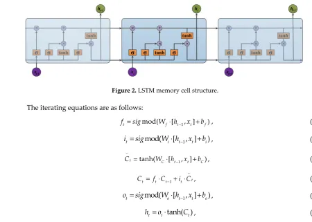
The serial version of HDFM achieves much better performance than the parallel version.
98
3) We collect communication signal data sets, which approximate the transmitted wireless
99
channel in the actual geographical environment. Such datasets are very useful for training networks
100
like CNNs and LSTM.
101
The rest of this paper is organized as follows. Section II briefly introduces the related works.
102
Section III introduces the principle of digital modulation signal and deep learning classification
103
methods. Section IV presents the experiments and analysis. Section V summarizes the paper.
104
2. Related Works
105
AMC is a typical multi-classification problem in the field of communication. This section
106
briefly introduces several feature extraction and classification methods in the traditional AMC
107
system. The CNN and LSTM models are also presented.
108
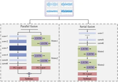
2.1. Conventional works based on separated feature and classifiers
109
Traditionally the feature and classifier are separately built for an AMC system. For example,
110
the envelope amplitude of signal, the power spectral variance of signal, and the mean of absolute
111
value signal frequency, was extracted in [11] to describe the signal from several different aspects.
112
Yang and Soliman used the phase probability density function for AMC [12]. Meanwhile,
113
traditional methods usually combine instantaneous and statistical characteristics. Shermeh used the
114
fusion of high-order moments and cumulants with instantaneous characteristics for AMC [13]-[14].
115
The features can describe the signals using both absolute and relative levels. In addition, the
116
high-order characteristics can eliminate the effects of noise. The sixth and eighth statistics are
117
widely used in several methods.
118
Classical algorithms have been widely used in the AMC system. Panagiotou et al. considered
119
AMC as a multiple-hypothesis test problem and used decision theory to obtain the results [15].
120
They assumed that the phase of AWGN was random and dealt with the signals as random variables
121
with the known probability distribution. Finally, the generalized likelihood ratio test or the average
122
likelihood ratio test was used to obtain the classification results by the threshold. The classifiers
123
were then used in the AMC system. In [16], shallow neural networks and SVM were used as
124
classifiers. In [17]-[18], modulation modes were classified using CNNs with high-level abstract
125
learning capabilities.
126
However, the traditional classifiers either need preprocessing to extract features or rely on the
127
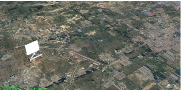
detailed prior information. This approach has led to negative influences of the classification
128
performance.
2.2. CNN – based methods
131
Advantage of CNNs is achieved with local connections and tied weights followed by some
132
form of pooling which results in translation invariant features. Furthermore, another benefit is that
133
they have many fewer parameters than fully connected networks with the same number of hidden
134
units. In [9], the authors treat the communication signal as a 2 dimensional data which similar to an
135
image and take it as a matrix to a narrow 2D CNN for AMC. They study the adaptation of CNN to
136
the time domain IQ data. A 3D CNN was used in [19]-[20] to process video information. The result
137
showed that CNN multi-frames were considerably more suitable than a single-frame network for
138
video cognition. In [21], Luan et al propose a Gabor Convolutional Networks, which combines
139
Gabor filters and CNN model, to enhance the resistance of deep learned features to the orientation
140
and scale changes. Recently, Zhang et al apply one-two-one network to compression artifacts
141
reduction in remote sensing [22]. This motivates us to solve the AMC problem.
142
2.3. LSTM – based methods
143
Various models have been used to process sequential signal, such as hidden semi-Markov
144
models [23], conditional random fields [24], and finite-state machines [25]. Recently, RNN became
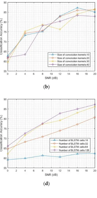
145
well-known with the development of deep learning. As a special RNN, LSTM has been widely used
146
in the field of voice and video because of its ability to handle gradient disappearance in traditional
147
RNNs. It has the less conditional independence hypothesis compared with the previous models and
148
facilitates integration with other deep learning networks. Researchers have recently combined
149
spatial/optical flow CNN features with vanilla LSTM models for global temporal modeling of
150
videos [26]-[30]. These studies have demonstrated that deep learning models have a significant
151
effect on action recognition [27], [29], [31] and video description [30], [32]. But to our best of
152
knowledge, the fusion of CNN and LSTM is never investigated to solve the AMC problem.
153
3. Heterogeneous Deep Model Fusion
154
3.1. Digital modulation signal description
155
The received signal in the communication system can be expressed as follows:
156
= ⋅ +
( ) ( ) ( ) ( )
y t x t c t n t , (1)
157
where x t( ) is the efficient signal from the transmitter, c t( ) represents the transmitted wireless
158
channel on the basis of the actual geographical environment, and n t( ) denotes the AWGN. The
159
digital modulation signals x t( ) can be expressed as follows:
160
π +θ π θ π θ
= + ( 2 ) − = + − + − ≤ ≤
( ) ( c s) j ft ( ) ( ccos(2 ) ssin(2 )) ( ), 0
x t A jA e g t nT A ft A ft g t nT t NT, (2)
161
where Ac and As are the amplitudes of the in-phase and quadrature channel, respectively; f
162
stands for the center frequency; θ is the initial phase of the carrier; and g t( −nT) represents the
163
digital sampling pulse signal. In the case of ASK, FSK, and PSK, As is zero. In accordance with the
164
digital baseband information, ASK, FSK, and PSK change Ac, f , and θ in the range of 0−M,
165
−
1 M, and 0 2 /− π M, respectively, with time. By contrast, QAM fully utilizes the orthogonality of
166
the signal. After dividing the digital baseband into I and Q channels, the information is
167
integrated into two identical frequency carriers with phase difference of 90° using ASK modulation
168
mode, which significantly improves the bandwidth efficiency.
169
As one of the most common noise, AWGN is always true whether or not the signal is in the
170
communication system. The power spectrum density is a constant at all frequencies, and the noise
171
amplitude obeys the Gauss distribution.
3.2. CNNs
175
CNNs are a hierarchical neural network that contains convolution, activation, and pooling
176
layers. In this study, the input of the CNN model is the data of signal time-domain waveform. The
177
difference among the classes of modulation methods is deeply characterized by the stacking of
178
multiple convolutional layers and nonlinear activation. Different from the CNN models in the
179
image domain, we use a series of one-dimensional convolution kernels to process the signals.
180
Each convolution layer is composed of a number of kernels with the same size. The
181
convolution kernel is common in each sample; thus, each kernel can be called a feature extraction
182
unit. This method of sharing parameters can effectively reduce the number of learning parameters.
183
Moreover, the feature extracted from convolution remains in the original signal position, which
184
preserves the temporal relationship well within the signal. In this paper, ReLU is used as the
185
activation function. We do not use the pooling layer for dimensionality reduction because the
186
amount of signal information is relatively small.
187
3.3. LSTM
188
Traditional RNNs are unable to connect the information as the gap grows. The vanishing
189
gradient can be interpreted as the forgetting of the human brain. LSTM overcomes this drawback
190
using gate structures that optimize the information transfer among memory cells. The particular
191
structures in memory cells include the input, output, and forget gates. An LSTM memory cell is
192
shown in Figure 2.
193
t h
t
x
t-1 h
t-1 x
t+1
h
t+1
x
194
Figure 2. LSTM memory cell structure.
195
The iterating equations are as follows:
196
−
= mod( ⋅[ 1, ]+ )
t f t t f
f sig W h x b , (3)
197
−
= mod( ⋅[ 1, ]+ )
t i t t i
i sig W h x b , (4)
198
−
= ⋅ +
1
tanh( [ , ] )
t C t t C
C W h x b , (5)
199
−
= ⋅ 1+ ⋅t
t t t t
C f C i C , (6)
200
−
= mod( ⋅[ 1, ]+ )
t o t t o
o sig W h x b , (7)
201
= ⋅tanh( )
t t t
h o C , (8)
202
where W is the weight matrix; b is the bias vector; i, f , and o are the outputs of the input,
203
forget, and output gates, respectively; C and h are the cell activations and cell output vectors,
204
respectively; and sigmod and tanh are nonlinear activation functions.
205
Standard LSTM usually models the temporal data in the backward direction but ignores the
206
forward temporal data, which has a positive impact on the results. In this paper, a method based on
207
bidirectional LSTM (Bi-LSTM) is exploited to realize AMC. The core concept is to use a forward and
a backward LSTM to train a sample simultaneously. Similarly, the architecture of Bi-LSTM network
209
is designed to model the time domain waveforms from past and future.
210
3.4. Fusion model based on CNN and LSTM
211
The HDMFs are established based on the fusion model in serial and parallel ways to enhance
212
the classification performance. The specific structure of the fusion model is shown in Figure 3.
213
214
Figure 3. Fusion model structure of HDMF in parallel and series modes. We note that two HDMF
215
models are used separately to solve the AMC problem.
216
The modulated communication signal has local special change characteristics. Meanwhile, the
217
data has temporal characteristics similar to voice and video. The fusion models exploit
218
complementary advantages on the basis of these two features.
219
The six layers of CNNs are used to characterize the differences between the digital modulation
220
modes in the fusion model. The kernel numbers of the convolutional layer are different for each
221
layer. The number of convolutional kernel in the first three layers increases gradually, which
222
transforms the single-channel into multi-channel signal data. Such a transformation also helps to
223
obtain effective features. Conversely, the number of convolutional kernel in the remaining layers
224
reduces gradually. Finally, the result is restored to a single-channel data. Although the data format
225
is same as the original signal, local features of the signal are extracted by multiple convolution
226
kernels. This leads to the representation for the final classification based on CNNs. The remaining
227
part of the fusion model uses the two-layer Bi-LSTM network to learn the temporal correlation of
228
signals. The output of the upper Bi-LSTM is used as the input of the next layer.
229
The parallel fusion model (HDMF). The two networks are used to train samples
230
simultaneously. The output of each network is then transformed into an 11-dimensional feature
231
vector by the full connection layer. The resulting feature vectors represent the judgment of the
232
modulation modes of the training samples by the two networks. We then combine the two vectors
233
based on the sum operation as:
234
ω ω
= ⋅ + ⋅
total c c l l, (9)
235
and,
ω ωc+ l =1,0≤ ≤ω 1, (10)
237
The loss function of parallel fusion model consists of two parts, which are balanced by the given
238
parameters.
239
Algorithm 1: Training HDMF(parallel)
1: Initialize the parameters θc in CNN, θl in LSTM, W, ω in the loss layer, the learning rate
μ, and the number of iteration t=0. 2: While the loss does not converge, do 3: t t= +1
4: Compute the total loss by total= ⋅ + ⋅ωc c ωl l.
5: Compute the backpropagation error ∂ ∂ total
i
x for each xi by ω ω
∂ = ⋅∂ + ⋅∂
∂ ∂ ∂
total c l
c l
i i i
x x x .
6: Update parameter W by − ⋅μ ∂ = − ⋅ ⋅μ ω ∂ − ⋅ ⋅μ ω ∂
∂ ∂ ∂
total c l
c l
W W
W W W
7: Update parameters ωc and ωl by ω μ ω
∂ − ⋅
∂ ,
,
,
c l c l
c l
.
8: Update parameter θ by θ μ
θ
∂ ∂
− ⋅ ⋅
∂ ∂
, ,,
m c l i
c l i
i c l
x
x .
9: End while
The serial fusion method (HDMF). It is similar to the encoder–decoder framework. In this
240
study, the encoding process is implemented by CNNs, afterwards LSTM decodes the corresponding
241
information. The features are extracted by the two networks, from simple representation to complex
242
concepts. The upper convolutional layers can extract features locally. Then, the Bi-LSTM layers learn
243
temporal characteristic from these representations.
244
For both kinds of fusion models, the final feature vectors are the probabilistic output of the
245
softmax layer. The fusion models are trained in the end-to-end way even when different neural
246
networks are used to address the AMC problem.
247
3.5. Implementation details and backpropagation
248
249
Figure 4. The geographic simulation environment.
250
The geographic simulation environment is shown in Figure 4, based on which we collect our
251
datasets. We captured the unmanned aerial vehicle communication signal data set, which is
252
developed by us based on STK, visual studio and MATLAB. We use TensorFlow [33] to design our
deep models. The Adam method [34] is used to solve our model with 0.001 learning rate. The
254
iterations are as follows:
255
μ − μ
= ⋅ 1+ − ⋅(1 )
t t t
m m g, (11)
256
ν − ν
= ⋅ + − ⋅ 2
1 (1 )
t t t
n n g , (12)
257
μ ∧ = − 1 t t t mm , (13)
258
ν ∧ = − 1 t t t nn , (14)
259
θ η ε ∧ ∧ Δ = − ⋅ + t t m n, (15)
260
where mt and nt are the first and second moment estimations of the gradient, which represent the
261
estimation of E g( )t and
2
( t)
E g , respectively; m∧t and
∧
t
n are the corrections of mt and nt ,
262
respectively, which can be regarded as the unbiased estimation of expectation; Δθ is the dynamic
263
constraint of learning rate; and μ, ν, ε, and η are constants.
264
The fundamental loss and the softmax functions are defined as follows:
265
= −
( , )x y log(py), (16)
266
+
+ = =
=
1T y i y
y i i
T
i j i j
W x b z
y z n W x b j i
e e
p
e e , (17)
267
where x is the input, y is the corresponding truth label, and zi is the input for the softmax layer.
268
The gradient of backpropagation is calculated as follows:
269
∂
∂ ∂
= = ⋅ = − − = −
∂ ∂ ∂
1
( )
y
t y jy j j jy
j y j y
p
g p I p p I
z p z p , (18)
270
where Ijy=1 if j=y, and Ijy=0 if j≠y.
271
4. Results
272
4.1. Classification accuracy of CNN and LSTM models
273
When CNNs and LSTM solve the AMC problem, the classification accuracies of CNNs are
274
reported with varying convolution layer depth from 1 to 4, the number of convolution kernels from
275
8 to 64, and the size of convolution kernels from 10 to 40. The classification accuracies of Bi-LSTM are
276
tested when varying layer depth from 1 to 3 and number of memory cells from 16 to 128. Bi-LSTM
277
used in the fusion model contains two layers. The number of convolution layers is 6. The number of
278
convolution kernels in the first three layers is 8, 16, and 32, and the size of the convolution kernel is
279
10. The number of convolution kernels in the remaining layers is 16, 8, and 1, and the size of the
280
convolution kernel is 20. The Bi-LSTM model consists of two layers with 128 memory cells.
(a) (b)
(c) (d)
(e)
Figure 5. Classification accuracy of CNN and LSTM models. (a) Classification accuracy of CNN with the
282
number of convolution kernels from 8 to 64; (b) Classification accuracy of CNN with the size of convolution
283
kernels from 10 to 40; (c) Classification accuracy of CNN with the number of convolution layers from 1 to 4; (d)
284
Classification accuracy of Bi-LSTM with the number of memory cells from 16 to 128; (e) Classification accuracy of
285
Bi-LSTM with the number of hidden layers from 1 to 3.
286
When SNR is set from 0 dB to 20 dB, the classification accuracy of CNN and Bi-LSTM models
287
is shown in Figure 5. The samples with SNR below 0 dB are not considered in this study. The
288
classification results of the CNN models are shown in Figure 5a–c. The average classification
289
accuracy of the CNN model for AMC can reach 75% with SNR from 0 dB to 20 dB. An excess of the
convolution kernels in each layer reduces the classification accuracy. The performance is better with
291
the number of convolution kernels from 8 to 32. The CNN models with the size of convolution
292
kernels from 10 to 40 have more or less the same classification accuracy. Increasing the number of
293
convolution layers from 1 to 3 results in a performance boost. The classification results of the
294
Bi-LSTM models are shown in Figure 5d–e. The results show that the Bi-LSTM model is more
295
suitable for AMC than the CNN model. The average classification accuracy of Bi-LSTM is 77.5%,
296
which is 1.5% higher than that of the CNN model. The performance is better with the number of
297
memory cells from 32 to 128 than others. The Bi-LSTM models with the number of hidden layers
298
more than 2 have essentially the same classification accuracy.
299
4.2. Comparison of classification accuracy between the deep learning models and the traditional method
300
We have compared five methods, including both traditional and deep learning methods, based
301
on the same data sets. The classification performance is as follows.
302
Table 1. Classification accuracy of different methods without noise.
303
Methods Wavelet + SVM CNN Bi-LSTM Parallel fusion Serial fusion
Accuracy 92.8% 91.2% 92.5% 93.1% 98.9%
Table 2. Classification accuracy of different methods with SNR from 0 to 20dB
304
SNR
Methods 20 dB 16 dB 12 dB 8 dB 4 dB 0 dB Wavelet+SVM 85.2% 84.1% 83.2% 81.6% 79.0% 77.5%
CNN 86.1% 84.0% 82.1% 78.1% 73.6% 62.1% Bi-LSTM 87.2% 84.9% 82.7% 77.5% 72.5% 66.0% Parallel fusion 89.1% 85.2% 84.6% 80.0% 75.4% 67.9%
Serial fusion 98.2% 95.6% 94.3% 91.5% 86.2% 78.5%
(a) (b)
Figure 6. Comparison of classification accuracy between the deep learning models and the
305
traditional method. (a) Classification accuracy of different methods without noise; (b) Classification accuracy
306
of different methods with SNR from 0 dB to 20 dB.
307
The modified classifiers are established based on the fusion model in serial and parallel modes
308
to increase the classification accuracy. As a result, we compare the classification accuracy of the
309
methods on the basis of deep learning with the traditional method by using wavelet and SVM
310
classifiers. The results are shown in Tables 1 and 2 and Figure 6. The results reveal that the fusion
311
methods have a significant effect on improving classification accuracy. The average classification
312
accuracy of parallel fusion model is 93% without noise, which is equal to the traditional method.
The classification accuracy of the parallel fusion model is 2% higher than the CNN model and 1%
314
higher than the Bi-LSTM model. Moreover, the average classification accuracy of the serial fusion
315
model is 99% without noise, which is 6% higher than the parallel fusion model. In fact, the fusion
316
methods are more beneficial to the classification accuracy with the SNR from 0 dB to 20 dB
317
compared with the noise-free situation. The average classification accuracy of the serial fusion
318
method is 91%, which is 11% higher than the parallel fusion method.
319
The performances of the classifiers show that deep learning achieves high classification
320
accuracy for AMC. Waveform local variation and temporal characteristics can be used to identify
321
modulation modes. In comparison with CNN and Bi-LSTM, the performance of the HDMF methods
322
is improved significantly because the classifiers can recognize the two features simultaneously.
323
However, the performance of the serial fusion is considerably higher than that of the parallel fusion
324
because the parallel method belongs to the decision-level fusion. The fusion can be viewed as a
325
simple voting process for results. The serial method belongs to the feature-level fusion, which
326
combines the two feature information to obtain the classification results.
327
(a) (b)
(c)
Figure 7. Confusion matrix of series fusion model. (a) Confusion matrix of series fusion model for 20 dB
328
SNR; (b) Confusion matrix of series fusion model for 10 dB SNR; (c) Confusion matrix of series fusion model for
329
0 dB SNR.
330
In this study, the modulation mode of the samples includes two forms, namely, within-class
331
and between-class modes. The confusion matrices show the identification results of the modulation
332
modes by serial fusion model when the SNR is 20, 10, and 0 dB, respectively; the results are shown
333
in Figure 7. When the SNR is 20 dB, a profound discrepancy is observed between the different
modulation modes. The confusion result does not have the error. The decrease of SNR, PSK, and
335
QAM is prone to misclassification within class, which is caused by the subtle differences in M-ary
336
phase mode. Moreover, representing the phase difference by waveform amplitude is not evident.
337
Furthermore, QAM can be considered as a combination of ASK and PSK in practice. The classifier
338
can detect the different types of changes simultaneously even when the result is incorrect at low
339
SNR. Therefore, only within-class misclassifications occur in the results.
340
5. Conclusions
341
In this study, we proposed the methods on the basis of deep learning to address the AMC
342
problem in the field of communication. The classification methods are end-to-end processes, which
343
reduce the additional steps to extract signal features compared with the traditional methods. First,
344
the communication signal data set system is developed based on the actual geographical
345
environment to provide the basis for related classification tasks. CNNs and LSTM are then used to
346
solve the AMC problem compared with the traditional method. Furthermore, the modified
347
classifiers based on the fusion model in serial and parallel modes are of great benefit to improve
348
classification accuracy with the SNR from 0 dB to 20 dB. The serial fusion mode has the best
349
performance compared with other modes. The confusion matrices significantly reflect the
350
shortcomings of the classifiers in this study. We will overcome these shortcomings and further
351
research on AMC in the future.
352
Acknowledgments: This work is supported by the National Natural Science Foundation of China (Grant no.
353
91538204).
References
356
1. M. Zheleva, R. Chandra, A. Chowdhery, A. Kapoor, and P. Garnett, TX miner: Identifying transmitters in
357
real-world spectrum measurements, IEEE International Symposium on Dynamic Spectrum Access Networks
358
(DySPAN), Sept 2015, pp. 94–105.
359
2. S. S. Hong and S. R. Katti, Dof: A local wireless information plane, Proceedings of the ACM SIGCOMM
360
2011 Conference, ser. SIGCOMM ’11. New York, NY, USA: ACM, 2011, pp. 230–241.
361
3. O. A. Dobre, A. Abdi, Y. Bar-Ness, and W. Su, Survey of automatic modulation classification techniques:
362
classical approaches and new trends, IET Communications, vol. 1, no. 2, pp. 137–156, April 2007.
363
4. W. A. Gardner, Signal interception: a unifying theoretical framework for feature detection, IEEE
364
Transactions on Communications, vol. 36, no. 8, pp. 897–906, Aug 1988.
365
5. Z. Yu, Automatic modulation classification of communication signals, Ph.D. dissertation, Department of
366
Electrical and Computer Engineering, New Jersey Institute of Technology, 2006.
367
6. A. V. Dandawate and G. B. Giannakis, Statistical tests for presence of cyclostationarity, IEEE Transactions
368
on Signal Processing, vol. 42, no. 9, pp. 2355–2369, Sep 1994.
369
7. A. Fehske, J. Gaeddert, and J. H. Reed, A new approach to signal classification using spectral correlation
370
and neural networks, First IEEE International Symposium on New Frontiers in Dynamic Spectrum Access
371
Networks, 2005. Nov 2005, pp. 144–150.
372
8. Y. LeCun, Y. Bengio, and G. Hinton, Deep learning, Nature, vol. 521, no. 7553, pp. 436–444, May 2015.
373
9. T. J. O’Shea, J. Corgan, and T. C. Clancy, Convolutional radio modulation recognition networks,
374
International Conference on Engineering Applications of Neural Networks. Springer, 2016, pp. 213–226.
375
10. S. Hochreiter and J. Schmidhuber, Long short-term memory, Neural Computation, vol. 9, no. 8, pp. 1735–
376
1780, Nov. 1997.
377
11. J. Lopatka and M. Pedzisz, Automatic modulation classification using statistical moments and a fuzzy
378
classifier, Signal Processing Proceedings, 2000. WCCC-ICSP 2000. 5th International Conference on, 2000, pp.
379
1500-1506 vol.3.
380
12. Y. Yang and S. Soliman, Optimum classifier for M-ary PSK signals, Communications, 1991. ICC'91,
381
Conference Record. IEEE International Conference on, 1991, pp. 1693-1697.
382
13. A. E. Shermeh and R. Ghazalian, Recognition of communication signal types using genetic algorithm and
383
support vector machines based on the higher order statistics, Digital Signal Processing, vol. 20, pp.
384
1748-1757, Dec 2010.
385
14. A. E. Sherme, A novel method for automatic modulation recognition, Applied Soft Computing, vol. 12, pp.
386
453-461, 2012.
387
15. P. Panagiotou, A. Anastasopoulos, and A. Polydoros, Likelihood ratio tests for modulation classification,
388
MILCOM 2000. 21st Century Military Communications Conference Proceedings, 2000, pp. 670-674.
389
16. M. Wong and A. Nandi, Automatic digital modulation recognition using spectral and statistical features
390
with multi-layer perceptions, Signal Processing and its Applications, Sixth International, Symposium on. 2001,
391
2001, pp. 390-393.
392
17. I. A. Basheer and M. Hajmeer, Artificial neural networks: fundamentals, computing, design, and
393
application, Journal of Microbiological Methods, vol. 43, pp. 3-31, Dec 2000.
394
18. L. S. Iliadis and F. Maris, An artificial neural network model for mountainous water-resources
395
management: The case of Cyprus mountainous watersheds, Environmental Modelling & Software, vol. 22,
396
pp. 1066-1072, Jul 2007.
397
19. S. Ji, W. Xu, M. Yang, and K. Yu, 3d convolutional neural networks for human action recognition. IEEE
398
PAMI, 2013.
399
20. A. Karpathy, G. Toderici, S. Shetty, T. Leung, R. Sukthankar, and L. Fei-Fei. Large-scale video
400
classification with convolutional neural networks. CVPR, 2014.
401
21. S. Luan, B. Zhang, C. Chen, J. Han and J. Liu. Gabor Convolutional Networks. arXiv preprint arXiv: 1705.
402
01450, 2017.
403
22. Baochang Zhang, Jiaxin Gu, Chen Chen, Jungong Han, Xiangbo Su, Xianbin Cao, Jianzhuang Liu.
404
One-Two-One network for Compression Artifacts Reduction in Remote Sensing, ISPRS Journal of
405
Photogrammetry and Remote Sensing, 2018.
406
23. T. Duong, H. Bui, D. Phung, and S. Venkatesh. Activity recognition and abnormality detection with the
407
switching hidden semi-markov model. CVPR, 2005.
24. C. Sminchisescu, A. Kanaujia, Z. Li, and D. Metaxas. Conditional models for contextual human motion
409
recognition. ICCV, 2005.
410
25. N. Ikizler and D. Forsyth. Searching video for complex activities with finite state models. CVPR, 2007.
411
26. N. Srivastava, E. Mansimov, and R. Salakhutdinov. Unsupervised learning of video representations using
412
lstms. ICML, 2015.
413
27. J. Donahue, L. A. Hendricks, S. Guadarrama, M. Rohrbach, S. Venugopalan, K. Saenko, and T. Darrell.
414
Long-term recurrent convolutional networks for visual recognition and description. CVPR, 2015.
415
28. J. Y. Ng, M. J. Hausknecht, S. Vijayanarasimhan, O. Vinyals, R. Monga, and G. Toderici. Beyond short
416
snippets: Deep networks for video classification. CVPR, 2015.
417
29. Z. Wu, X. Wang, Y. Jiang, H. Ye, and X. Xue. Modeling spatial-temporal clues in a hybrid deep learning
418
framework for video classification. ACM Multimedia, 2015.
419
30. S. Venugopalan, M. Rohrbach, J. Donahue, R. J. Mooney, T. Darrell, and K. Saenko. Sequence to sequence -
420
video to text. ICCV, 2015.
421
31. S. Lazebnik, C. Schmid, and J. Ponce. Beyond bags of features: Spatial pyramid matching for recognizing
422
natural scene categories. CVPR, 2006.
423
32. L. Yao, A. Torabi, K. Cho, N. Ballas, C. Pal, H. Larochelle, and A. Courville. Describing videos by
424
exploiting temporal structure. ICCV, 2015.
425
33. M. Abadi, A. Agarwal, P. Barham, E. Brevdo, Z. Chen, C. Citro, G. S. Corrado, A. Davis, J. Dean, M. Devin
426
et al., Tensorflow: Large-scale machine learning on heterogeneous distributed systems, arXiv preprint
427
arXiv:1603.04467, 2016.
428
34. D. P. Kingma and J. Ba, Adam: A method for stochastic optimization, CoRR, [Online]. Available:
429
http://arxiv.org/abs/1412.6980.