Article
Quantification of the Energy Storage Contribution to
Security of Supply through the F-Factor methodology
Spyros Giannelos, Predrag Djapic, Danny Pudjianto and Goran Strbac
Department of Electrical and Electronic Engineering, Imperial College London, London SW7, 2AZ, UK; [email protected]; [email protected]; [email protected];
Abstract: The ongoing electrification of the heat and transport sectors is expected to lead to a substantial increase in peak electricity demand over the coming decades, which may drive significant investment in network reinforcement in order to maintain a secure supply of electricity to consumers. The traditional way of security provision has been based on conventional investments such as the upgrade of the capacity of electricity transmission or distribution lines. However, the energy storage technology can also provide security of supply, thereby constituting a cost-efficient alternative to expensive conventional reinforcements. In this context, the current paper presents a methodology for the economic quantification of the security contribution of energy storage. This methodology makes use of mathematical optimization for the calculation of the F-factor metric, which reflects the optimal amount of peak demand reduction as compared to the power capability of the energy storage asset. In this context, a case study is presented in which the security contribution of energy storage is analyzed as a function of its power capability, energy capacity and efficiency as well as of characteristics of load patterns.
Keywords: F-factors; energy storage; investments in electricity systems; mathematical optimization; security of supply.
1. Introduction
Energy Storage (ES) constitutes a technology that can provide a wide range of benefits to the electricity system operation and investment. Such benefits include strategic investment flexibility for the network planner to hedge against exogenous and endogenous uncertainty [1]-[2], support for the real-time balancing of electricity supply and demand [3] through the provision of ancillary services [4], decentralized coordination of distributed energy resources within microgrids [5] and provision of security of supply through reduction of peak demand [6]. Such benefits can enable greater penetration of low-carbon generation resources, which can have environmental benefits as well as economic ones [7] given that low-carbon generation is characterized by lower operating costs than conventional generation based on fossil fuels.
Traditionally, network security has been provided through investment in conventional assets, such as transformers and electricity transmission and distribution lines. Sufficient level of investment in these assets can improve the supply reliability of electricity to consumers by considering outages in designing the secured distribution system. With the advent of smart grid technologies, such as demand-side response and ES, the concept of security of supply is being updated to include such non-network solutions. The ability of ES to provide security of supply was first recognized in a study conducted by EPRI in 1976 [8] that dealt with the potential of pumped hydroelectric storage to ensure electricity supply while reducing investment in expensive conventional generation units.
There have been various attempts in the literature to quantify the ES security contribution. Authors in [9] make use of dynamic programming while [10] uses a probabilistic methodology based on chronological Monte Carlo simulations for computing the Effective Load Carrying Capability of an ES plant. Note that, as opposed to such approaches, the F-factor methodology does not take into consideration reliability parameters of grid assets such as mean time to repair or mean time before
failure. Rather F-factors focus on the maximum peak reduction achieved by a specific storage device, thereby constituting an initial indication for the security contribution of energy storage and that can be easily explained to management.
It is worth noting that despite the availability of methodologies for the quantification of ES security contribution, current network planning standards do not yet provide an explicit formal framework for its assessment. This is the case, for example, with Engineering Recommendation P2/6 [11], which is a distribution network planning standard followed by Distribution Network Operators in Great Britain. Although this planning standard explicitly recognizes the contribution of distributed generation to the security of supply, it does not include formal recognition of the contribution of ES. Hence, an update of the planning standards is necessary so that the security contribution of network solutions is properly evaluated. The economic assessment of each of the benefits that non-network technologies provide is necessary for the establishment of a level-playing field where candidate technologies for investment are compared as to their suitability for deployment based solely on their total economic benefit. For example, if deployment of energy storage yields greater total economic benefit than some conventional investment, then it will lead to a justified investment.
This paper presents an approach to quantify the security contribution of ES based on mathematical optimization for the evaluation of the F-factor metric. Such an approach offers an intuitive estimation of the capacity value of ES. In this context, the contributions of the present paper are as follows.
• Presentation of F-factors as a methodology for the quantification of the security contribution of ES.
• Demonstration of the mathematical formulation for the optimization problem that is solved for the evaluation of the F-factor metric.
• Sensitivity analysis of the security contribution of ES as a function of multiple quantities such as energy storage power capability, efficiency, energy capacity and characteristic of load patterns.
The paper is structured as follows. In section 2 , the methodology of F-factors is explained, and the associated mathematical formulation is presented. section 3 presents a case study that showcases the proposed methodology of F-factors and explains their dependence on technical characteristics of energy storage as well as on the load pattern. section 4 discusses the findings, while section 5 discusses future work pathways and concludes.
2. The F-Factor methodology
In the previous section, it was mentioned that the ES technology can bring various benefits to the electricity system including the provision of security of supply, the economic benefit of which can be evaluated using the F-factor methodology [12].
2.1. Definition of the metric
Figure 1. Illustration of an electricity load profile where its peak demand is reduced through the use of ES, which discharges during peak hours (i.e. acts as a generator of electricity) and charges during off-peak hours (i.e. acts as a load).
The current paper presents the application, for the first time, of the F-factor metric for the evaluation of the energy storage security contribution. Specifically, the F-factor metric is defined as the ratio of P, which stands for the optimal reduction in peak demand (kW), over C that stands for the power capability (kW) of the ES plant, as in equation (1). In this regard, this metric is dimensionless and is expressed in percentage terms.
𝐹 =𝑃
𝐶 (1)
From (1), it becomes obvious that to calculate the F-factor it is important to conduct an optimization study so as to obtain the maximum peak demand reduction 𝑃. The mathematical formulation for the corresponding optimization problem is provided in sub-section 2.2. . It is also evident that the F-factor metric depends on the characteristics of energy storage. Hence, it is also important to perform sensitivity analysis and examine how the F-factor measure is affected by the load characteristics, such as the shape of the demand profile, and characteristics of the energy storage, such as the efficiency and the time required for a full charge / discharge of the ES plant.
2.2. Optimization problem
The modelling approach for calculating the ES security contribution is based on obtaining the maximum amount of peak demand (kW) that can be reduced through solving the following deterministic linear and continuous optimization problem.
𝑚𝑖𝑛𝑖𝑚𝑖𝑧𝑒 𝑃𝑚𝑎𝑥 (2)
𝑃𝑚𝑎𝑥≥ 𝐷𝑡+ 𝑃𝑡𝑖𝑛− 𝑃𝑡𝑜𝑢𝑡 ∀ 𝑡 ∈ 𝑇 (3)
𝐸𝑡= 𝐸𝑡−1+ 𝛿 ∙ 𝜂 ∙ 𝑃𝑡𝑖𝑛− 𝛿 ∙ 𝑃𝑡𝑜𝑢𝑡 ∀ 𝑡 ∈ 𝑇∗ (4)
𝐸𝑡= 𝐼 ∙ 𝐸0+ 𝛿 ∙ 𝜂𝑃𝑡𝑖𝑛− 𝛿 ∙ 𝑃𝑡𝑜𝑢𝑡 𝑡 = 1 (5)
Power
Time Peak hours
Discharging energy
Charging energy
𝐸1− 𝐸𝑇 = 0 ∀𝑑 (6)
𝐸𝑡≤ 𝐸0 ∀ 𝑡 ∈ 𝑇 (7)
𝑃𝑡𝑖𝑛 ≤ 𝑃0 ∀ 𝑡 ∈ 𝑇 (8)
𝑃𝑡𝑜𝑢𝑡≤ 𝑃0 ∀ 𝑡 ∈ 𝑇 (9)
The objective function (2) aims to minimize the maximum net demand, which, by default, is greater than the net demand across all time periods (3). Net demand is defined as the summation of the initial demand 𝐷𝑡 (kW) with the power that charges the ES plant 𝑃𝑡𝑖𝑛 (kW), minus the power that gets discharged from the ES, 𝑃𝑡𝑜𝑢𝑡 (kW). As can be seen, there is no cost involved in the objective function. Rather, for the calculation of the F-factors, the objective of the storage device is to achieve minimization of the peak demand.
Constraint (4) models the operation of the ES device. Essentially, the state of charge (SOC) 𝐸𝑡 (kWh) at period t is equal to that at period t-1 plus the energy that charges the ES plant at period t minus the energy which gets discharged at the same period, where 𝜂 is the efficiency of charging (p.u.). Also, parameter 𝛿 (hours) represents the time-granularity of the load data. For example, it is 𝛿 = 0.5 for load-data where each period corresponds to half an hour or 𝛿 = 1 for hourly granularity. Essentially, this constraint models the fact that the ES operates as a load during off-peak periods (i.e. charging with energy) and as a generator (i.e. discharging) during peak times.
Constraint (5) is the application of (4) to the first time period. Notice that 𝐼 (p.u.) is a decision variable that specifies the initial SOC of the ES. Also, 𝐸0 is the storage capacity (kWh). Constraint (6) states the assumption that the SOC at the last period of the horizon is equal to the SOC at the first period. Constraint (7) specifies that the SOC must be less than or equal to the initial energy capacity 𝐸0 at all times. Similar limitations apply to the power capability. Specifically, the power that charges ES (8) and that which is discharged (9), at every time period, must be less than or equal to the maximum power capability 𝑃0. Note that the quantities 𝐸0 and 𝑃0 are connected via the equation 𝐸0= 𝜇𝑃0, where 𝜇 is the number of hours required for a complete charging or discharging of the ES plant.
3. Case Study: Evaluation of the ES security contribution via F-factors
Figure 2. Diagrams of two substations: a bulk supply point substation (e.g. 132/33 kV) and a primary substation (e.g. 33/11 kV), each of which supplies a load.
Figure 3. Normalized time-series for load profiles 1 and 2. The profiles span a period of seven days, with the fourth day being the one that exhibits the peak demand.
Sensitivity analysis is performed by running a series of studies, each of which involves solving the aforementioned optimization problem each time for a different combination of the following ES parameters: charging efficiency 𝜂, power capability 𝑃0 and energy capacity 𝐸0. The sensitivity analysis is performed by assuming two different durations for the study horizon. The first is when only the peak day (fourth day in Figure 3) is considered, while the second is when the entire 7-day period, as shown in Figure 3, is considered. By selecting two different durations, it is possible to evaluate how the length of the selected load profiles can affect the values for the F-factors. Note that the actual load profile for every hour of the respective period is evaluated by multiplying the normalized time series with the peak demand for the primary substation and the BSP respectively.
The results for each of the two load profiles are shown in Tables 1 and 2 below, with grey-coloured cells containing two values. At the top, the value for the F-factor corresponds to the case in which only the peak day is considered while the bottom value, shown in parentheses, corresponds to the entire 7-day period. White-coloured cells contain only one value for the F-factor since it is the same regardless of whether one day or the entire 7-day period is considered.
Note that the sensitivity analysis has been conducted by selecting values for the efficiency 𝜂 equal to 60%, 80% and 100%, for the power capability 𝑃0 equal to 10%, 20%, 30% and 50% of the peak demand of the corresponding load profile, and for parameter 𝜇 equal to 1 hour up to 8 hours. The studies are conducted through the use of the FICO Xpress optimization platform on a Xeon 3.46 GHz computer.
0 0.25 0.5 0.75 1
Table 1. F-factors for an ES unit connected to the primary substation (load profile 1). Grey-coloured cells contain, at the top, the F-factor when only the load profile corresponding to the peak day is considered, while the bottom value, shown in parentheses, corresponds to the entire 7-day period. White-coloured cells contain only one value for the F-factor and this value is the same for the peak day and for the entire 7-day period.
𝜇
𝑷𝟎 at 10% of peak 𝑷𝟎 at 20% of peak 𝑷𝟎 at 30% of peak 𝑷𝟎 at 50% of peak
Efficiency Efficiency Efficiency Efficiency
100% 80% 60% 100% 80% 60% 100% 80% 60% 100% 80% 60%
1h 62% 62% 62% 46% 46% 46% 37% 37% 37% 27% 27% 27%
2h 92% 92% 92% 61% 61% 61% 49% 49% 49% 37% 37% 37%
3h 100% 100% 100% 73% 73% 73% 59% 59% 59% 45% 45% 45%
4h 100% 100% 100% 84% 84% 84% 67% 67% 67% 52%
50%
(52%) 46%
(52%)
5h 100% 100% 100% 93% 93% 93% 74% 74%
73% (74%) 54% (59%) 50% (58%) 46% (55%)
6h 100% 100% 100% 100% 100%
96% (100%)
82% 82%
73% (82%) 54% (62%) 50% (59%) 46% (56%)
7h 100% 100% 100% 100% 100% 96%
(100%)
89% 82%
(89%) 73% (89%) 54% (63%) 50% (60%) 46% (57%)
8h 100% 100% 100% 100% 100% 96%
(100%) 90% (96%) 82% (96%) 73% (92%) 54% (64%) 50% (61%) 46% (58%)
Table 2. F-factors for an ES unit that is connected to the BSP substation characterized by load profile 2.
𝜇
𝑷𝟎 at 10% of peak 𝑷𝟎 at 20% of peak 𝑷𝟎 at 30% of peak 𝑷𝟎 at 50% of peak
Efficiency Efficiency Efficiency Efficiency
100% 80% 60% 100% 80% 60% 100% 80% 60% 100% 80% 60%
1h 49% 49% 49% 40% 40% 40% 34% 34% 34% 25% 25% 25%
2h 80% 80% 80% 58% 58% 58% 45% 45% 45% 33% 33% 33%
3h 100% 100% 100% 68% 68% 68% 53% 53% 53% 41% 41% 41%
4h 100% 100% 100% 76% 76% 76% 61% 61% 61% 48% 45%
(48%) 41%
(46%)
5h 100% 100% 100% 84% 84% 84% 68% 68%
6h 100% 100% 100% 91% 91%
87%
(91%)
75% 75%
66% (75%) 49% (56%) 45% (53%) 41% (50%)
7h 100% 100% 100% 98% 98%
87% (98%) 82% 75% (82%) 66% (78%) 49% (57%) 45% (54%) 41% (51%)
8h 100% 100% 100% 100%
98% (100%) 87% (100%) 82% (88%) 75% (85%) 66% (81%) 49% (58%) 45% (55%) 41% (52%)
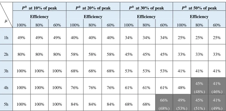
Figure 4 shows an example of storage operation aimed at peak minimization with application to load profile 2 during the peak day. The original time series, shown in blue colour, which has a peak of 170,363 kW, is minimized in terms of its peak through ES operation. The resulting time series is shown in red colour and has a peak of 128,695 kW, thereby achieving a 41,668 kW peak reduction. This case corresponds to an ES plant with have power capability equal to 50% of the peak demand of the initial profile, i.e. 85,181.5 kW and 100% efficiency, while requiring 8 hours for a full charge. Hence, the calculated F-factor is equal to (41,668)/ 85,181.5 = 49% (see Table 2).
Figure 4. Initial demand profile (in blue) and optimal demand profile (in red) following ES operation.
Figure 5 presents the net power inflow in the ES unit for the example presented in Figure 4. It can be seen that during periods when the initial load profile is relatively low the ES unit charges with energy (i.e. draws power acting as a load), while during peak periods the ES plant discharges the stored energy (shown in negative values).
Figure 5. Net power inflow (kW) in the ES unit.
Discussion on these results follows in the subsequent section.
4. Discussion
The results obtained in the previous section allow us to make key observations about the F-factors. First of all, the F-factors cannot increase as the energy storage power capability increases. This can be witnessed by observing the values of the F-factors from left to right across any row belonging to the above tables. The reason for such reduction in F-factors is based on the definition of the F-factor
0 20,000 40,000 60,000 80,000 100,000 120,000 140,000 160,000 180,000 Lo ad (k W)
Initial load profile (kW) Load profile (kW) after ES operation
metric as the ratio of the achieved peak demand reduction divided by the storage power capability. For example, regarding the first row of Table 1, for a storage asset connected to the primary substation characterized by load profile 1 (peak: 7,036 kW) , when the storage power capability is 10% of the peak (i.e. 703.6 kW), the achieved peak reduction is evaluated at 437.5 kW; hence the corresponding F-factor stands at 437.5 / 703.6 = 62% F-factor. However, when the storage power capability becomes three times larger, i.e. 30% of the peak (i.e. 2,110.8 kW), the achieved peak reduction, for the same efficiency, becomes 778.75 kW, thereby yielding an F-factor value equal to 37%. In other words, the increase in the achieved peak reduction is typically less than the increase in power capability. Hence, using a storage device with greater power capability does not entail greater security contribution, in percentage terms. Rather, the security contribution, expressed in the F-factor value, is seen to reduce. Furthermore, it is noticeable from within the tables that F-factors may stay the same as power capability increases. For example, for a duration 𝜇 of 6 – 8 hours in Table 1 ,the F-factor 100% does not reduce when moving from a 10% to 20% storage power capability. The reason for this lies in the fact that such high values for 𝜇 entail high energy storage capacity that allows the device to significantly contribute to peak reduction and utilize effectively its increased power capability.
A further observation that can be made is that F-factors increase as the full charge/discharge duration 𝜇 increases, until the storage unit has sufficient capacity after which additional capacity has no effect. This can be witnessed by observing the top of each of the columns in the above tables and moving downwards towards increasing values for 𝜇. The reason for this is that greater duration 𝜇 essentially translates to greater storage energy capacity (kWh), leading to greater potential for energy storage to contribute towards peak minimization and, as a result, correspond to greater F-Factor values.
Additionally, by comparing the values in Table1, which corresponds to the peaky profile, with those in Table2 it can be seen that the F-factors of the peaky profile 1 are higher than the corresponding ones of the less peaky profile 2. That is, the values in Table 1 are higher (or equal in the case of 100%) with the corresponding ones in Table 2. One of the main reasons for this is based on the shape of the load profiles and mainly on the shape of the peaks. For example, for a ‘peaky’ profile with a narrow peak of high magnitude, the peak can be reduced even with a small output from the storage unit, thereby providing significant security contribution. On the other hand, a ‘flatter’ profile that is characterized by a long period of high values for load and a small peak requires a storage unit with a significant amount of energy capacity in order to make significant security contribution. Such contribution largely depends on the difference in the height of the peak demand with the subsequent largest peaks; if a load profile has a peak that is much higher than the second-highest peak, then reducing the second-highest peak will provide considerable security contribution leading to a high value for the F-factor. Hence, there is more scope for the provision of security contribution on a peaky load profile than on a flatter one, like profile 2.
Notice that the F-factors for the peak day are equal to those for the 7-day period for most of the cases as shown in the white-colored cells in Table 1 and Table 2. However, there are cases, as shown in grey-colored cells, in which these two values are different from each other. The difference can be observed for storage units characterized by increased values for 𝜇 (i.e. increased storage capacity) and storage power capabilities. In these cases, the F-factors corresponding to the 7-day period are higher than those corresponding to the peak day only. The reason for this difference lies in the fact that as the storage capacity and power capability increase, the storage unit can charge with more energy, which can be drawn from a longer period of time i.e. from a week rather than from the peak day only, thereby allowing for greater reduction of peak demand, which contributes to enhanced security of supply.
the storage capacity increases (high value of 𝜇) as well as its power capability, the efficiency starts playing a role because the storage unit has significant ability to reduce the peak demand, and this ability can be affected at low efficiencies, since in such cases it would to draw extra amount of power to charge, which could lead to extra peaks in the load profile.
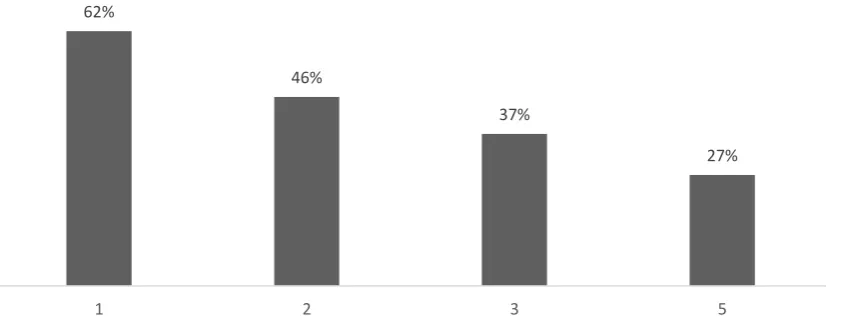
Finally, it is interesting to note that when more than one storage units are connected to the same bus, the F-factor of the total storage capacity is a non-increasing function of the number of these connected ES units. This essentially means that increased investment in storage per bus does not increase the contribution to the security of supply provided by the combined investment capacity. This can be shown by selecting any type of storage unit from the above tables. For instance, it is found in Table 1 that a 100% efficient storage unit with power capability equal to 10% of the peak demand and with 1h duration has an F-factor equal to 62% (see row 1 and column 1 in Table 1). That is, when only such a storage unit is connected to the primary substation, its F-factor is 62% . On the other hand, when two storage units of this type are connected to the primary substation, their combined power capability is equal to 10% + 10% of the peak demand, which means that it is equivalent to having connected one unit of the same type but with twice the power capability. Such a unit provides an F-factor value equal to 46% as can be observed in Table 1 (row 1, column 4). In the same vein, when three such units are connected to the same bus, the F-factor for the combined storage capacity is equal to 37% (row1, column 7 in Table 1) and with five such units, the combined F-factor is equal to 27% (row 1, column 10 in Table 1). Hence, investing in increased storage capacity at a bus leads to reduced F-factor for the combined storage system because, according to (1), the achieved peak demand reduction is less than the increase in the total storage power capability.
Figure 6. The values on the horizontal axis indicate the number of identical ES units connected to the same bus. The height of the bars illustrates the corresponding F-factor value.
5. Conclusions and future work
This paper presents the F-factor methodology for the economic evaluation of the security contribution of energy storage units. The F-factor metric is defined as the ratio of the maximum reduction in peak demand divided by the power capability of the ES plant. A mathematical optimization problem is presented for obtaining the maximum peak reduction, thereby allowing for the estimation of the F-factor values. The value of the F-factor is shown to be a function of the ES power rating, its energy capacity and its ES efficiency of charging as well as of the shape of the demand curve. Notably, F-factors tend to increase with an increase in ES efficiency and they also increase as the full charge/discharge duration of the ES asset increases.
Future work includes the study of the F-factor metric within a larger network consisting of many buses and lines and different voltage levels as well as a range of smart technologies such as demand-side response and soft open points [14]. Finally, it is of interest to the authors to investigate the
62%
46%
37%
27%
1 2 3 5
security contribution of different types of ES technologies, including thermal energy storage, pumped hydroelectric storage and flywheel [15] energy storage.
Acknowledgement
The authors are grateful for the valuable support and funding received from the European
Union’s Horizon 2020 research and innovation programme under grant agreement No 773505 for the
“Pan-European system with an efficient, coordinated use of flexibilities for the integration of a large share of RES” (EU-SysFlex project); further information about the project can be found at https://eu-sysflex.com/. All contents and views expressed in this paper are the sole responsibility of the authors and do not necessarily express the views of the EU-Sysflex consortium.
References
1. S. Giannelos; I. Konstantelos; G. Strbac, “Option value of dynamic line rating and storage”, in IEEE EnergyCon, 2018, pp. 1-6.
2. S. Giannelos; I. Konstantelos; G. Strbac, "Option Value of Demand-Side Response Schemes Under Decision-Dependent Uncertainty", in IEEE Transactions on Power Systems, vol. 33, no. 5, pp. 5103-5113, Sept. 2018. 3. D. Pudjianto; M. Aunedi; P. Djapic; G. Strbac, “Whole-Systems Assessment of the Value of Energy Storage
in Low-Carbon Electricity Systems”, in IEEE Transactions on Smart Grid, 2014, vol. 5, no. 2, pp. 1098-1109. 4. R. Moreno; R. Moreira; G. Strbac“, A MILP model for optimizing multi-service portfolios of distributed
energy storage”, in Applied Energy, 2015.
5. D. Papadaskalopoulos, D. Pudjianto and G. Strbac, “Decentralized Coordination of Microgrids with Flexible Demand and Energy Storage”, in IEEE Transactions on Sustainable Energy, vol.5, no.4, pp. 1406-1414, October 2014.
6. S. Agamah; L. Ekonomou, “Energy storage system scheduling for peak demand reduction using evolutionary combinatorial optimization”, in Sustainable Energy Technologies and Assessments, 2017, pp 73– 82.
7. G. Strbac; M. Aunedi; I. Konstantelos; R. Moreira; F. Teng; R. Moreno; D. Pudjianto; A. Laguna; P. Papadopoulos, “Opportunities for Energy Storage: Assessing Whole-System Economic Benefits of Energy Storage in Future Electricity Systems”, in IEEE Power and Energy Magazine, 2017, vol. 15, no. 5, pp. 32-41. 8. Public Service Electric and Gas Company, Electric Power Research Institute, “An assessment of energy
storage systems suitable for use by electric utilities”, Final report. 1979.
9. R. Sioshansi; S.H. Madaeni; P. Denholm, “A dynamic programming approach to estimate the capacity value of energy storage”, in IEEE Transactions on Power Systems. 2014.
10. I. Konstantelos; G. Strbac, “Capacity value of energy storage in distribution networks”, in The Journal of Energy Storage, 2018.
11. Electricity Networks Association, “Engineering Recommendation P2/6: Security of Supply”, 2006.
12. R. Allan; G. Strbac; P. Djapic; K. Jarrett, “Developing the P2/6 Methodology”, University of Manchester, 2004. 13. Electricity Networks Association, “Engineering Report 130 Working Group. Substation demand profiles”,
2013-2018.
14. S. Giannelos; I. Konstantelos; G. Strbac, "Option value of Soft Open Points in distribution networks," in IEEE Eindhoven PowerTech, Eindhoven, 2015, pp. 1-6.