Type of the Paper (Publication)
1
Medical video coding based on 2nd generation
2
wavelets: Performance evaluation
3
M Ferroukhi1, A Ouahabi2*, M Attari1, Y Habchi3, M Beladgham3, A Taleb-Ahmed4
4
1 Laboratory of Instrumentation, Faculty of Electronics and Computers, University of Sciences and Technology
5
Houari Boumediene, Algiers.
6
2 Polytech Tours, Brain and Imaging INSERM U930, University of Tours, Tours, France.
7
3 Electrical Engineering Department, Bechar University, Algeria.
8
4 LAMIH CNRS U 8201, Valenciennes University, France. Affiliation 1; [email protected]
9
* Correspondence: [email protected] ; Tel.: +33603894463
10
11
Abstract: The operations of digitization, transmission and storage of medical data, particularly
12
images require increasingly effective encoding methods not only in terms of compression ratio and
13
flow of information but also in terms of visual quality. At first, there was DCT (discrete cosine
14
transform) then DWT (discrete wavelet transform) and their associated standards in terms of coding
15
and image compression. After that, the 2nd generation wavelets seeks to be positioned and
16
confronted to the image and video coding methods currently used. It is in this context that we
17
suggested a method combining bandelets and SPIHT (set partitioning in hierarchical trees)
18
algorithm. There are two main reasons for our approach: the first lies in the nature of the bandelet
19
transform to take advantage by capturing the geometrical complexity of the image structure. The
20
second reason stems in the suitability of encoding the bandelet coefficients by the SPIHT encoder.
21
Quality measurements shows that in some cases (for low bit rates) the performances of the proposed
22
coding compete with the well-established ones and opens up new application prospects in the field
23
of medical imaging.
24
Keywords: Bandelet; medical imaging; quadtree decomposition; SPIHT coder; video coding; video
25
quality measure.
26
27
1. Introduction and motivation
28
The huge amount of patient medical data recorded at every moment in hospitals, medical
29
imaging centers and others medical organizations have become a major issue. The need for
30
quasi-infinite storage space and efficient real-time transmission in specific applications such as
31
medical imaging, military imaging and satellite imaging requires advanced techniques and
32
technologies including coding methods to reduce the amount of data to be stored or transmitted.
33
Without coding of information, it is very difficult and sometimes impossible to make a way to store or
34
communicate big data (large volumes of high velocity and complex images, audio and video
35
information) via the internet. The encoding of these data is obtained by eliminating the redundant or
36
unnecessary information in the original frame which can’t be identified with the naked eye.
37
38
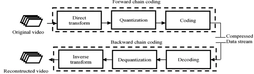
Figure 1 recalls the key steps of video coding:
39
Transformation is a linear and reversible operation that allows the image to be represented in the
40
transform domain where the useful information is well localized. This property will make it possible
41
during the compression to achieve good discrimination, that is to say the suppression of unnecessary
42
or redundant information. The discrete cosine transform and the wavelet transform are among the
43
most popular transforms proposed for image and video coding.
44
Quantization is the step of the compression process during which a large part of the elimination
45
of unnecessary or redundant information occurs.
46
Coding techniques e.g. Huffman coding and arithmetic coding [16-18] are the best-known
47
entropy coding particularly in image and video coding.
48
49
Figure 1.Simplified video coding scheme
50
51
It is well known that lossless compression methods have the advantage of providing an image
52
without any loss of quality and the disadvantage of compressing weakly. Hence, this type of
53
compression is not suitable for transmission or storage of big data such as video. Conversely, lossy
54
compression produces significantly smaller file sizes often at the expense of image quality. However,
55
lossy coding based on transforms has gained great importance when several applications have
56
appeared. In particular, lossy coding represents an acceptable option for coding medical images. E.g.,
57
DICOM (Digital Imaging Communication in Medicine) JPEG based on DCT and DICOM JPEG 2000
58
based on wavelet. In this context, wavelet-based image coding, e.g. JPEG2000, using multiresolution
59
analysis [1-2] exhibits performance that is highly superior to other methods such as those based on
60
discrete cosine transform (DCT), e.g. JPEG.
61
In 1993, Shapiro introduced a lossy image compression algorithm that he called embedded
62
zerotrees of wavelet (EZW) [3]. The success of coding wavelet approaches is largely due to the
63
occurrence of effective subband coders. The EZW encoder is the first to provide remarkable
64
distortion-rate performance while allowing progressive decoding of the image. The principle of
65
zerotrees, or other partitioning structures in sets of zeros, makes it possible to take account of the
66
residual dependence of the coefficients between them. More precisely, since the high-energy
67
coefficients are spatially grouped, their position is effectively computed by indicating the position of
68
the sets of low energy coefficients. After separation of the low energy coefficients and the energetic
69
coefficients, the latter is relatively independent and can be efficiently coded using quantification and
70
entropy coding techniques.
71
In 1996, Said and Pearlman proposed a hierarchical tree partitioning coding scheme called set
72
partitioning in hierarchical tree (SPIHT) [4], based on the same basic EZW, and exhibiting better
73
performance than the original EZW.
74
Video compression algorithms such as MPEG-4 and H.264 use inter-frame prediction to reduce
75
video data between a series of images. This involves techniques such as differential coding where an
76
image is compared with a reference image and only the pixels that have changed with respect to that
77
reference image are coded.
78
MPEG allows to encode video using three coding modes:
79
Intra coded frames (I): frames are coded separately without reference to previous images (i.e. as
80
JPEG coding).
81
Predictive coded frames (P): images are described by difference from previous images.
82
Bidirectionally predictive coded frames (B): the images are described by difference with the
83
previous image and the following image.
In order to optimize MPEG coding, the image sequences are in practice coded in a series of I, B,
85
and P images, the order of which has been determined experimentally. The typical sequence called
86
GOP (Group of Pictures) is as follows:
87
88
Figure 2.Typical sequence with I, B and P frames.
89
P frame can only refer to the previous I or P frames, while a B frame can refer to previous or subsequent I or
90
P frames.
91
92
To evaluate the visual quality of the reconstructed video, several measurements of the quality of
93
the MPEG video are validated in [5-6].
94
As a successor to the famous H.264 or MPEG-4 standards [7-8], HEVC (High Efficiency Video
95
Coding) or H.265 standard has recently been defined as a promising standard for video coding, In
96
June 2013 [9], the first version of HEVC was announced, and to improve the efficiency of the coding of
97
this standard, a set of its components requires more development. In addition, this new system
98
requires new hardware and software investments delaying its adoption in applications such as in the
99
medical field.
100
This work is motivated by the prospect to offer Our motivation lies in the prospect of offering a
101
new codec that is simple to implement with performances superior to the current H264 standard and
102
which could compete with the H265 or HEVC standard for some applications. This superiority is
103
based on the SPIHT algorithm and the second-generation wavelets.
104
One can ask: “Why using second generation wavelets (instead of classical wavelets)?”
105
This new generation of wavelets makes it possible to generate decorrelated coefficients, and to
106
eliminate any redundancy by retaining only the necessary information and it is better suited to
107
geometric data (ridges, contours, curves, or singularities). This 2nd generation wavelets consists of
108
Xlets such as shearlets, bandelets, curvelets, contourlets, ridgelets, noiselets, contourlets, etc. These
109
Xlets provide interesting performance in some applications, i.g. contourlets-based denoising [10],
110
contourlets-based video coding [11-12], curvelets-based contrast enhancement [13], bandelets-based
111
geometric image representations [14], shearlets-based image denoising [15], …
112
In this paper, we analyse and compare to the current state-of-the-art coding methods, the
113
performances of a new coding method based on bandelet transform where its coefficients are encoded
114
using the set partitioning in hierarchical trees (SPIHT).
115
The remainder of this paper is organized as follows: Section 2 presents and recalls the main
116
properties of bandelet transform and Section 3 introduces bandelet-SPIHT-based video coding.
117
Section 4 focuses on the experimental aspect and the analysis of the results. It should be noted that
118
some preliminary results published recently in IEEE IECON 2016 [19] have been completed and
119
analyzed in order to point out the advantages but also the limitations of the proposed method.
120
Finally, Section 5 concludes this study.
122
123
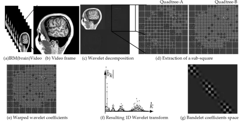
Figure 3.Example of graphical steps of the bandelet transformation algorithm
124
2. Bandelet transform algorithm
125
2.1. Bandelet transform
126
In order to organize intra- and inter-frames interactions, we choose the threshold to control the
127
coding rate of the algorithm.
128
In step 2, 2D orthogonal or bi-orthogonal bandelet basis are performed to the original image.
129
The bandelization is implemented in the following steps.
130
Step 3:
131
- Performing dyadic square by recursive split of the original wavelet transform.
132
- Figure 3 graphically summarizes the main steps of bandelet transform illustrated on a brain
133
MRI frame.
134
- Select each split dyadic square.
135
1D discrete wavelet transform is performed and stored in 2D image of the same size as projected
136
result of the sampling location along potential directions and sorting 1D points result from left to
137
right. The correct threshold and the good direction acquire a smaller approximation error.
138
To control the error between the recovered and the original signals for a fixed number of
139
parameters (number of bits, quantization step and Lagrangian multiplier), a Lagrangian function is
140
used to provide optimal direction A better bandelet is, indeed, defined by minimizing a Lagrangian
141
cost function. Moreover, the Lagrangian minimization requests no information on regularity.
142
The zigzag scanning order is used in low-scale to aggregate wavelet coefficients in the
143
upper-left corner of the output square.
144
2.2. Geometric flows
145
The bandelet bases are based on an association between the wavelet decomposition and an
146
estimation of the image information of geometric character. The estimation of the geometry is done by
147
studying the contours present in an image. A contour is then seen as a parametric curve that will be
148
characterized by its tangents. To do this, we look for gradients of significant importance in the frame.
149
Around each region of frames, the local geometry directions, in which the frame has regular
150
variations in the neighborhood of each pixel, are determined by two-dimensional geometric flow of a
151
vector field, instead to describe the geometry of the frames through edges.
153
Figure 4. Example of quadtree decomposition
154
2.3. Quadtree division process
155
In the discussed algorithm, on each dyadic square and scale, we apply the bandelet transform; it
156
is evidently a redundant transformation. The best segmentation represented as a quadtree is obtained
157
by the using of the Lagrangian optimization. An example of a quadtree area division is shown in
158
Figure 3.
159
In order to minimize the distortion rate, we use a parallel vertical or horizontal flux in each
160
dyadic square. The macro block is considered regular uniformly, in the case where there is no
161
geometric flow and the wavelet basis is used. Otherwise, deformed wavelets replaced wavelet bases,
162
as explained in [20-21].
163
All directions in each block acquired by quadtree decomposition are tested, where for a given
164
quantization step the best quadtree requires a minimization of Lagrangian.
165
(
)
2 2
(
)
( )
1d d dR jS jG jB
j
L f , R = f - f +λQ R + R + R
166
where
167
:
d
f The original signal.
168
:
dR
f The recovered signal using inverse 1D wavelet transform.
169
:
jS
R The bits number needed to encode the dyadic segmentation.
170
:
jG
R The bits number needed to encode the geometric parameter.
171
:
jB
R The bits number needed to encode the quantized bandelets coefficients.
172
:
λ
The Lagrangian multiplier is chosen to be equal to3 28,for a justification of this value see [22].173
:
Q The quantization step.
174
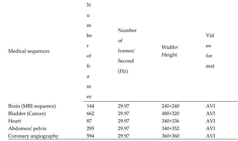
Table 1. Details and characteristics of all standards tested video
175
Medical sequences
N
u
m
be
r
of
fr
a
m
es
Number
of
frames/
Second
(Hz)
Width× Height
Vid
eo
for
mat
Brain (MRI sequence) 144 29.97 240×240 AVI Bladder (Cancer) 662 29.97 480×320 AVI
Heart 87 29.97 340×336 AVI
Abdomen/ pelvis Coronary angiography
295 594
29.97 29.97
340×352 360×360
AVI AVI
The following steps implement the quadtree structure.
177
For each dyadic square the value of the Lagrangian is restricted to
178
• Initialize the quadtree with the square of size and initialize
179
• are the fourth sub-squares defended for each square and
180
is the Lagrangian of the sub-tree
181
• The sub-squares should be merged if . If so, declare as a leaf and record
182
the optimal geometry. Update .
183
Repeat the previous step for each square of size 2L.
184
2.4. Warped wavelet along geometric flows
185
In order to perform the complex geometry and remove the redundancy of orthogonal wavelet
186
coefficients, bandelet basis decomposition is applied with a fast application of the geometric
187
flow, quadtree decomposition, warping and bandeletization.
188
In each dyadic square at each scale, the geometric flow it used to warp the wavelet basis along
189
the direction regularity. After warping, the next step is to construct bandelets by applying a
190
bandeletization procedure.
191
The function of wavelet includes high-pass filters and the vanishing moments at lower
192
resolutions, this is valid for vertical and diagonal detail coefficients, but not for horizontal
193
detail coefficients. The problem of regularity along the geometric flow is due to the function of
194
scaling where it includes low-pass filters and does not have the vanishing moment at lower
195
resolutions.
196
To take advantage of regularity along the geometric flow for horizontal detail coefficients, the
197
deformed wavelet basis is bandeletized by replacing the horizontal wavelet with modified
198
horizontal wavelet function. In near of singularity, the wavelets coefficients correlations are
199
removed by using bandeletization operation.
200
201
(a).Wavelet (b). Bandelet
202
Figure 1. Analyses histogram of bandelet and wavelet coefficient values
203
204
205
After warping and bandeletization operations, the regions are regular along the vertical or
206
horizontal direction. In the end, warped wavelets are used to compute bandelet coefficients with 1D
207
discrete wavelet transform than are encoded using SPIHT coder.
208
S L S = L f , R
( )
(
d)
S :S L L S0
( )
.(
S1,S2,S3,S4)
S,( )
( )
( )
( )
( )
20 1 0 2 0 3 0 4
'
L S = L S + L S + L S + L S +λQ
( )
< '( )
L S L S S
( )
(
( ) ( )
)
0 '
L S = min L S , L S
S
-300 -200 -100 0 100 200 300
0 200 400 600 800 1000 1200 1400 1600 1800
Wavelet coefficients values
W
avel
et
c
oef
fici
en
ts
num
ber
-3000 -200 -100 0 100 200 300
500 1000 1500 2000 2500 3000 3500 4000
Bandelet coefficient values
B
and
el
et
coe
ffi
ci
ent nu
m
The next section is based on the principal that the most significant coefficients are achieved by
209
the bandelet transform. In the applications of time constraints, this result confirms that our approach
210
can be used.
211
Figure 4 illustrates this feature and compares wavelet and bandelet coefficients histograms
212
results. Therefore, the SPIHT encoder, primarily applied to the wavelet results, will become
213
Bandelet-SPIHT in this contribution.
214
3. Process of encoding
215
SPIHT algorithm [4] is one of the most efficient encoder nowadays, were it used in many
216
applications [23-24]; whose special performances show its outperform to the JPEG 2000 in many
217
practical situations. The list of effectiveness values symbols, are not used by SPIHT encoder such as
218
EZW [25].
219
The SPIHT algorithm takes up the principles evoked in EZW while proposing to recursively
220
partition the coefficient trees. Thus, where EZW encodes an isolated insignificant coefficient, SPIHT
221
performs a recursive partitioning of the tree so as to determine the position of the significant
222
coefficients in the descendant of the considered coefficient. The significant coefficients are coded
223
similarly to EZW: their sign is sent as soon as they are identified as significant coefficients and they
224
are added to the list of coefficients to be refined.
225
This algorithm also works by bit planes. The Bits sent during the significance pass correspond to
226
the program executed at the encoder during the execution of the classification algorithm of significant
227
and insignificant coefficients. By following the same program, the decoder remains synchronous with
228
the decisions of the encoder and finds the same classification.
229
In each pass of SPIHT, the only wavelet coefficients are encoded with magnitudes exceeding a
230
certain halved threshold values where is defined as:
231
( )
( )
2
2
n p
i, j
T = , n = log max c i, j (2)
232
Where:
233
p = 0,1,..., P denote the number pass
234
( )
c i, j is the coefficient at position
( )
i, j in frame.235
The coefficients sets are ordered in spatial orientation trees, with roots in the lowest frequency
236
subband.
237
The following is the three descending nodes set to correspond to wavelet coefficients at
238
coordinates
( )
i, j :239
• Offspring set denoted by O i, j
( )
in the same spatial orientation. Except for lowest level240
nodes that have four offspring.
241
• Type A set denoted byD i, j
( )
.242
• Type B set (excluding the offspring) denoted byL i, j = D i, j - O i, j
( )
( ) ( )
.243
The resulting bandelet coefficients are ordered according to the its test of significance and
244
stored in three separate sets of lists: list of insignificant sets (LIS), list of insignificant pixels (LIP)
245
and list of significant pixels.
246
During the initialization step, added pixels to LIP are tested, added descendants sets to LIS are
247
sequentially assessed and significant pixels are stored in initial empty list LSP.
248
The coding operation being with LIP, if pixels are insignificant, it stays in LIP; otherwise, pixels
249
moved towards LSP.
250
Also for LIS, insignificant pixels stay in LIS. The significant pixels are divided into significant
251
A-type set where will be divided into B-type set and four pixels; type B set is added to the end
252
of LIS, while the remainders are examined for significance.
253
The principal proposed coding method is formulated as follows:
254
• Step1: Medical videos input
255
• Step2: Performing 2D discrete wavelet transform to decompose sequences into a subband.
• Step3: Decompose the frame recursively into the equal squares
257
• Step4: The geometric flow is applied to the each square.
258
• Step5: Warping the discrete wavelets along the geometric flux.
259
• Step6: Perform the 1D discrete wavelet transform to bandelize the wavelet bases.
260
• Step7: SPIHT encoded the resulting bandelets coefficients.
261
262
263
Figure 5.Medical video used for assessment
264
(a) Bladder cancer; (b) Heart; (c) Abdomen/Pelvis; (d) Coronary angiography.
265
266
• Step8: Gauging the quality of the recovered video sequences according to both
267
objective and subjective criterions.
268
269
4. Experimental results
270
We proposed in this work, a new algorithm for medical video coding based on the bandelet
271
transform coupled by SPIHT coder that detect complex geometric and reduce different existing
272
redundancy in video.
273
The accuracy of the algorithm is tested in a bit-rate range varies from 0.1 to 0.5Mbps on some
274
sized medical video sequences; each sequence has variable number of frames, and frame rate equal to
275
29.97 frames/second. The set tested medical videos are illustrated in Figure 5.
276
The perceived quality of recovered frames has been measured. Moreover, a comparison between
277
Bandelet-SPIHT and the wavelet transform using SPIHT encoder, MPEG-4, and H.26x, showed
278
promising results.
279
4.1. Warped wavelet along geometric flows
280
The characteristic of the multimedia services quality is summarized in a single term of the quality
281
of the experience [26-27], especially, with the appearance of digital video coding, storage, and
282
transmission systems and their fundamental limitations in the measuring the quality of video.
283
The National Telecommunications and Information Administration (NTIA) is one of the
284
pioneered organizations were it general models for estimating video quality [28], it is adopted with
285
the American National Standards Institute (ANSI) and included in The International
286
Telecommunication Union (ITU) as a normative method [29]. Also, this domain recognized other
287
organizations were having performed major research efforts [30-31].
288
The objective metrics are used to judge the performance of proposed algorithm and the higher quality
289
of the reconstructed frames is measured [32-34].
290
291
(a)
(b)
(c)
(d)
(a)
(b)
(c)
(d)
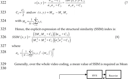
292
Figure 6. Block diagram of the SSIM measurement system
293
The peak signal-to-noise ratio (PSNR) represents an objective evaluation parameter for the
294
measurement of image quality, is defined as follows:
295
(
)
( )
1 0 2 1 2 n-PS N R = 1 0 lo g
M S E
296
where
297
• is the dynamic of the signal (the maximum possible value for a pixel). In the
298
standard case of an image where the components of a pixel are coded on bits,
299
• MSE represents the mean square error between two frames, namely the original frame and
300
the recovered frame of size and is given by
301
( ) ( )
(
)
2( )
1 1
3
M N ri = j =
1
MSE = f i, j - f i, j
MN
302
The PSNR is an easy, fast and very popular quality measurement metric, widely used to compare the
303
quality of video encoding and decoding. Although a high PSNR generally means a good quality
304
reconstruction, but this is not always the case. Indeed, PSNR requires original image for comparison,
305
but this may not be available in every case, also PSNR does not correlate well with subjective video
306
quality measures, so is not very suitable for perceived visual quality [35]. Hence, the interest in
307
considering a measure of structural similarity (SSIM) adapted to the human visual system. SSIM
308
index introduces three key features: luminance contrast and structure This metrics is defined in (4)
309
and the block diagram of the SSIM measurement system is represented in Fig 6:
310
( )
1( )
2 2 1 2 5 x y x y
M M +C l x, y =
M + M +C
311
where
312
x
M and My are the mean intensity of the signal and y defined by and
313
1
N y i i = 1M = y
N respectively.
314
Ci=Ki2D2 , i =1,2, and Ki is a constant, such asKi << 1and is the dynamic range of the pixel values
315
( corresponds to a grey-scale digital image when the number of bits/pixel is 8).
316
The contrast comparison function takes the following form:
317
( )
2( )
2 2 2 2 6 x y x y
σ σ +C
c x, y =
σ +σ +C
318
where
319
320
The structure comparison function is defined as follows:
321
(
2n −1)
8
n =
(
2n − =1)
255.x 1 1 N x i i M x N = =
D 255 D = c( )
(
2 2)
1 21 1 1 = = − −
Nx i x
i
x M
N
σ
( )
3( )
3( )
3 3
7 xy
x y x y
σ +C cov x, y +C
s x, y = =
σ σ +C σ σ +C
322
and
323
with
324
Hence, the explicit expression of the structural similarity (SSIM) index is:
325
( )
(
(
1)(
)(
2)
)
( )
2 2 2 2
2
2 2
8
x y xy
x y 1 x y
M M +C σ +C
SSIM x, y =
M + M +C σ σ +C
326
where
327
328
Generally, over the whole video coding, a mean value of SSIM is required as Mean SSIM (MSSIM):
329
330
331
Figure 7. Diagram of the visual information fidelity (VIF) metric.
332
(
)
(
)
( )
1
9
Lr i ri
i = 1
MSSIM f, f = SSIM f , f L
333
where and are the contents of frames (original and recovered respectively) at the ith local
334
window (or sub-image), and is the total of local windows number in frame.
335
The MSSIM values exhibit greater consistency with the visual quality.
336
In 2006, Sheikh and Bovik [36] proposed a new paradigm for video quality assessment: information
337
video fidelity (VIF). This criterion quantifies the Shannon information that is shared between the
338
original and recovered images relatively to the contained information in the original image itself. It
339
uses natural scene statistics modelling in conjunction with an image-degradation model and a human
340
visual system (HVS) model.
341
Visual Information Fidelity uses the Gaussian scale mixture model (GSM) in the wavelet domain. To
342
obtain VIF one performs a scale-space-orientation wavelet decomposition using the steerable pyramid
343
and models each subband in the source as , where is a random field of scalars and is a
344
Gaussian vector.
345
The distortion model is where is a scalar gain field and is an additive Gaussian noise.
346
VIF then assumes that the distorted and source images pass through the human visual system
347
and the HVS uncertainty is modelled as visual noise and for the source and distorted image
348
respectively.
349
The model is then:
350
Reference signal E = C + N
( )
10351
Test signal F = D + N
( )
11352
Where and denote the visual signal at the output of the HVS model from the reference and
353
the test videos respectively, from which the brain extracts cognitive information.
354
The VIF measure takes values between 0 and 1, where 1 means perfect quality and is given by:
355
2
3 2
C
C = cov ( x , y )=Mxy −M Mx y
1 1
1
N
xy i i
i
M x y
N =
= −
( )
( )
1 2 2 2 1
1 1 =
= −
−
N
xy i i xy
i
x y M
N
σ
C = SU
E F
C
Test
D
F
Frame Distortion HVS Recevier
E
HVS Recevier
(
)
(
)
( )
12
j j j
j
j j j
j
I C ; F s VIF =
I C ; E s
356
357
a. Original b. GALL5/3 filter c. CDF9/7 filter
358
FFigure8.Recovered frames using:
359
(b). Bandelet(GALL5/3)-SPIHT and (c). Bandelet(CDF9/7)-SPIHT at 0.2Mbps.
360
where, is the conditional mutual information between andY ,givenz; denotes the
361
random field from a channel in the original image, is a realization of for a particular image and
362
the index runs through all the sub bands in the decomposed image.
363
4.2. Choice of the perfect filter and transform
364
In this part, MRI video is encoded with performing of the Bandelet-SPIHT algorithm for various
365
bit rates. Pixels resolution MRI images is made using different filters, where each with its own
366
peculiar properties (filter orders, symmetry and compact support) has been investigated. In order to
367
find the best objective measures filter for video compression, the pioneer biorthogonal families was
368
considered, thus the wavelets CDF9/7 (Cohen-Daubechies-Feauveau) and GALL5/3 (GENERATING
369
ANY LEVELS LE) are used, they part of the family of symmetric biorthogonal wavelets CDF.
370
The choices of these filters are for their simplicity, symmetry and for the support width. CDF9/7
371
and GALL5/3 are characterized with (9/7, 2) and (5/3, 4), respectively.
372
where (I/J, K), I/J and K showing the number of coefficients in decomposition low-pass filter
373
(analysis)/ reconstitution high pass filter (synthesis) and number of vanishing moments [37-40].
374
After an accurate visual inspection of the images in Figure 8, we adopt the bi-orthonormal
375
wavelets CDF9/7 rather GALL5/3 to reduce the artifacts levels. The results obtained show that the
376
visual quality of the recovered frame using the Bandelet algorithm (CDF9/7) + SPIHT is close to the
377
original frame.
378
On the other hand, we notice a presence of fuzzy areas in the case of the use of GALL5/3 filter,
379
which is arduous to detect by a simple observation.
380
Comparative results between (Bandelet+SPIHT) algorithm and (Wavelet +SPIHT) applied to coronary
381
angiography test frame at various bit rates are illustrated in Figure9.
382
383
Figure9. Performance evaluation of Bandelet-SPIHT versus (Wavelet) SPIHT in terms of objective
384
parameters.
385
(
)
I X ;Y z X C
j
s Sj
j
0.1 0.15 0.2 0.25 0.3 0.35 0.4 0.45 0.5 10
15 20 25 30 35 40
BITRATE(Mbps)
PSN
R
(d
B
)
Wavelet-SPIHT Bandelet-SPIHT
0.1 0.15 0.2 0.25 0.3 0.35 0.4 0.45 0.5 0.4
0.5 0.6 0.7 0.8 0.9 1
BITRATE(Mbps)
MS
S
IM
Wavelet-SPIHT Bandelet-SPIHT
0.1 0.15 0.2 0.25 0.3 0.35 0.4 0.45 0.5 0
0.1 0.2 0.3 0.4 0.5 0.6 0.7 0.8
BITRATE(Mbps)
VI
F
386
387
388
(a) (b) (c) (d)
389
Figure 10. Comparative quality assessments medical video using Bandelet(CDF9/7)-SPIHT (Top
390
row), and Wavelet(CDF9/7)-SPIHT (Bottom row) at 0.5 Mbps
391
Figure10, shows the visual results for tested medical video. From this figures, it is clearer that the
392
performance of (Bandelet+SPIHT), indicates that our algorithm gives best results compared to the
393
conventional and state-of-the art coding methods and it is an apt tool to detect all special complex
394
geometric.
395
While the discrete wavelet transform (SPIHT algorithm) is subject to blocking artifacts
396
397
F Figure 11. Comparison PSNR(dB) between the existing coding standards and proposed coding method
398
4.3. Bandelet-SPIHT versus standards encoder comparison
399
To check and prove the efficiency of the algorithm, more comparison with H.26x and MPEG
400
standards are required. The H.264 and H.265 are known standards especially in the security industry.
401
It is interesting to examine the maximum PSNR (dB) at the output of the proposed algorithm. As
402
illustrated in Figure 11, the proposed method demonstrates its relatively better performance
403
compared to the standard video coding H.264 and H.265 in terms of PSNR. For example, under
404
2Mbps it is clearly seen that the PSNR curves of the proposed algorithm is significantly outperformed
405
0 500 1000 1500 2000 2500
29 30 31 32 33 34 35 36 37 38 39
BITRATE(Kbps)
PSN
R
(d
B
)
to the conventional standards encoders. Furthermore, for low bit rates (e.g. 1Mbps) our method can
406
exceed H.264 and H.265 encoders by 2.41 dB and 0.23 dB respectively. Moreover, the PSNR
407
improvements are more significant in high values.
408
5. Conclusion
409
The objective motivating our study was to propose a coding method with high performances in
410
terms of visual quality and PSNR at low bit rates. Bandelets using SPIHT encoder is an effective
411
condidate meeting the specific requirements of our application in the medical field and particulary in
412
medical imaging where the quality of the image at low bit rates is a major requirement for the
413
practitioner.
414
In order to show the efficiency of Bandelet-SPIHT algorithm, a set of medical sequences as test
415
examples is considered. At low bit rates, Bandelet-SPIHT algorithm gives significantly better results
416
(PSNR and visual quality) comparing to some cutting-edge coding techniques such as H.26x family
417
(namely H.264 and H.265).
418
From this point of view, the expected goal is achieved and the prospects for application in
419
medical imaging are promising.
420
Geometric image compression methods are a very dynamic search direction. One could mention
421
the construction of transformations that adapt automatically to the geometry without the need to
422
specify it or discrete geometry approaches ... They all agree, however, that geometry is the key to
423
significantly improve current compression methods.
424
425
Author Contributions: Methodology, Abdeldjalil OuahabiI; Project administration, Abdelmalik Taleb-Amed;
426
Software, Merzak Ferroukhi and Yacine Habchi; Supervision, Mokhtar Attari; Validation, Mohamed
427
Beladgham.
428
429
References
430
[1] A.Ouahabi, Signal and Image Multiresolution Analysis, Wiley-ISTE: Hoboken, NJ, USA, 2012.
431
[2] S.Mallat, A Wavelet Tour of Signal Processing: A Sparse Way, Academic Press, third ed., USA, 2009.
432
[3] J.M.Shapiro, Embedded image coding using zerotrees of wavelet coefficients, IEEE Transactions on Signal
433
Processing. 41 (1993) 3445-3462.
434
[4] A.Said, W.Pearlman, A new fast and efficient image codec based on set partitioning in hierarchical trees, IEEE
435
Transactions on Circuits and Systems for Video Technology. 6 (1996) 243-250.
436
[5] G.W.Cermak, S.Wolf, E.P.Tweedy, M.H.Pinson, A.A.Webster, Validating objective measures of MPEG video
437
quality, SMPTE Journal. 107 (2015) 226-235.
438
[6] Y.Q. Shi, S.Huifang, Image and Video Compression for Multimedia Engineering: Fundamentals, Algorithms,
439
and Standards, second ed., CRC Press, 2000.
440
[7] G.J.Sullivan, J.R.Ohm, W.Han, T.Wiegand, Overview of the high efficiency video coding (HEVC) standard, IEEE
441
Trans on Circuits and Systems for Video Technology. 22 (2012) 1649-1668.
442
[8] J.R.Ohm, G.J.Sullivan, H.Schwarz, T.K.Tan, T.Wiegand, Comparison of the coding efficiency of video coding
443
standards-including high efficiency video coding (HEVC), IEEE Trans on Circuits and Systems for Video
444
Technology. 22 (2012) 1669-1684.
445
[9] ITU-T Recommendation H.265, High Efficiency Video Coding, 2013.
446
[10] S.Sidahmed, Z.Messali, A.Ouahabi, S.Trépout, C.Messaoudi, S.Marco, Nonparametric denoising methods based
447
on contourlet transform with sharp frequency localization: Application to electron microscopy images with low
448
exposure time, Entropy Journal. 17 (2015) 2781-2799.
[11] S.Katsigiannis, G.Papaioannou, D.Maroulis, A contourlet transform based algorithm for real-time video
450
encoding, SPIE Photonics Europe, Real-Time Image and Video processing Conference, Brussels, Belgium. 8437
451
(2012).
452
[12] Z.Shu, Y.Luo, G.Liu, Z.Xie, Arbitrarily shape object-based video coding technology by wavelet-based contourlet
453
transform, IEEE International Conference on Information and Automation, Aug 2015.
454
[13] J.L.Starck, F.Murtagh, E.J.Candès, D.L.Donoho, Gray and color image contrast enhancement by the curvelet
455
transform, IEEE Transactions on Image Processing. 12 (2003) 706-717.
456
[14] E.Le Pennec, S.Mallat, Sparse geometric image representations with bandelets, IEEE Transactions on Image
457
Processing. 14 (2005) 423-438.
458
[15] G.Xie, X.Qu, J.Yan, Bandelet image coding based on SPIHT, 2nd International Symposium on Information
459
Technologies and Applications in Education (ISITAE). (2008) 297-301.
460
[16] P.G.Howard, J.S.Vitter, Parallel lossless image compression using Huffman and arithmetic coding, Proceedings
461
of the IEEE Data Compression Conference, Snowbird,March 1992.
462
[17] P.N.Tudor, MPEG-2 video compression, Electronics & Communication EngineeringJournal. 7 (1995) 257-264.
463
[18] R.Mateosian, Introduction to data compression, IEEE Micro, 16 (1996) 78.
464
[19] Y.Habchi, A.Ouahabi, M.Beladgham, A.Taleb-Ahmed, Towards a new standard in medical video compression,
465
The 42nd Annual Conference of the IEEE Industrial Electronics Society (IECON2016), October 2016.
466
[20] G.Peyre, S.Mallat, Surface compression with geometric bandelets, ACM Transactions on Graphics. 24 (2005)
467
601-608.
468
[21] G.Peyre, S.Mallat, Discrete bandelets with geometric orthogonal filters, IEEE International Conference on Image
469
Processing (ICIP). 1 (2005) 65-86.
470
[22] E. Le Pennec,S. Mallat, Sparse geometrical image approximation with bandelets, IEEE Transaction on Image
471
Processing, 2004.
472
[23] S.K.Mukhopadhyay, S.Mitra, M.Mitra, An ECG signal compression technique using ASCII character encoding,
473
Measurement Journal. 45 (2012) 1651-1660.
474
[24] S.Chang, L.Carin, A modified SPIHT algorithm for image coding with a joint MSE and classification distortion
475
measure, IEEE Transactions on Image Processing. 15 (2006) 713-725.
476
[25] B.Rani, R.K.Bansal, S.Bansal, Comparative analysis of wavelet filters using objective quality measures, IEEE
477
International Advance Computing Conference. (2009) 402-407.
478
[26] S.Winkler, P.Mohandas, The evolution of video quality measurement: from psnr to hybrid metrics, IEEE
479
Ransactions on Broadcasting. 54 (2008) 660-668.
480
[27] S.Winkler, Digital Video Quality Vision Models and Metrics, John Wiley & Sons, first ed, 2005.
481
[28] S.Wolf, Features for automated quality assessment of digitally transmitted video, NTIA Report 264, June 1990.
482
[29] H.P.Margaret, S.Wolf, A new standardized method for objectively measuring video quality, IEEE Transactions
483
on Broadcasting. 50 (2004) 312-322.
484
[30] D.Hands, A basic multimedia quality model, IEEE Transactions on Multimedia. 6 (2004) 806-816.
485
[31] A.Watson, J.Hu, J.Mcgowan, DVQ: A digital video quality metric based on human vision, Journal of Electronic
486
Imaging. 10 (2001) 20-29.
487
[32] Z.Wang, A.C.Bovik, H.R.Sheikh, E.P.Simoncelli, Image quality assessment: from error visibility to structural
488
similarity, IEEE Transactions on Image Processing. 13 (2004) 600-612.
[33] H.R.Sheikh, A.C.Bovik, Image information and visual quality, IEEE Transactions on Image Processing. 15 (2006)
490
430-444.
491
[34] M.Mark, S.Grgic, M.Grgic, Picture quality measures in image compression systems, IEEE Region 8 EUROCON.
492
COMPUTER AS A TOOL. 2 (2003) 233-237.
493
[35] N.Yamsang, S.Udomhunsakul, Image quality scale (IQS) for compressed images quality measurement,
494
Proceedings of the International MultiConference of Engineers and Computer Scientists IMECS. 9 (2009)
495
789-794.
496
[36] M.Trupti, S.D.Ruikar, Selection of wavelet for satellite image compression using picture quality measures,
497
International Conference on Communication and Signal Processing. (2013) 1003-1006.
498
[37] F.Adamo, G.Andria, F.Attivissimo, A.M.L.Lanzolla, M.Spadavecchia, A comparative study on mother wavelet
499
selection in ultrasound image denoising, Measurement Journal. 46 (2013) 2447-2456.
500
[38] G.Andria, F.Attivissimo, G.Cavone, N.Giaquinto, A.M.L.Lanzolla, Linear filtering of 2-D wavelet coefficients for
501
denoising ultrasound medical images, Measurement Journal. 45 (2012) 1792–1800.
502
[39] L.Angrisani, P.Daponte, Thin thickness measurements by means of a wavelet transform-based Method,
503
Measurement Journal. 20 (1997) 227-242.
504
[40] E.Dumic, S.Grgic, M.Grgic, New image-quality measure based on wavelets, Journal of Electronic Imaging. 19
505
(2010) 011018.