Earth Surf. Dynam., 7, 895–910, 2019 https://doi.org/10.5194/esurf-7-895-2019 © Author(s) 2019. This work is distributed under the Creative Commons Attribution 4.0 License.
Mapping landscape connectivity as a driver of species
richness under tectonic and climatic forcing
Tristan Salles1, Patrice Rey1, and Enrico Bertuzzo2
1School of Geosciences, University of Sydney, Sydney, NSW, 2006, Australia
2Dipartimento di Scienze Ambientali, Informatica e Statistica, Università Ca’Foscari Venezia, Venice, Italy
Correspondence:Tristan Salles (tristan.salles@sydney.edu.au)
Received: 13 June 2019 – Discussion started: 26 June 2019
Revised: 12 August 2019 – Accepted: 7 September 2019 – Published: 1 October 2019
Abstract. Species distribution and richness ultimately result from complex interactions between biological, physical, and environmental factors. It has been recently shown for a static natural landscape that the elevational connectivity, which measures the proximity of a site to others with similar habitats, is a key physical driver of local species richness. Here we examine changes in elevational connectivity during mountain building using a landscape evolution model. We find that under uniform tectonic and variable climatic forcing, connectivity peaks at mid-elevations when the landscape reaches its geomorphic steady state and that the orographic effect on geomorphic evolution tends to favour lower connectivity on leeward-facing catchments. Statistical comparisons between connectivity distribution and results from a metacommunity model confirm that to the 1st order, land-scape elevation connectivity explains species richness in simulated mountainous regions. Our results also predict that low-connectivity areas which favour isolation, a driver for in situ speciation, are distributed across the entire elevational range for simulated orogenic cycles. Adjustments of catchment morphology after the cessation of tectonic activity should reduce speciation by decreasing the number of isolated regions.
1 Introduction
The idea that mountainous landscapes play a role in biolog-ical evolution has a long history that can be tracked back to Darwin and Wallace, when fauna boundaries were noted to correspond to physiographic discontinuities and gradi-ents (Wallace, 1860). Over geological timescales (millions of years), surface processes including erosion and incision conspire to undo surface uplift driven by tectonic and geo-dynamic processes. These competing processes can convert landscapes of low elevation and relief, a homogeneous envi-ronment, and low resistance to migration into complex land-scapes with sharp environmental gradients and fragmented habitats separated by migratory corridors (Steinbauer et al., 2016).
Several studies have shown that on geological timescales, changes in landscape morphology stimulate migratory be-haviour, dispersal, and redistribution as species track their optimum habitats (Gillespie and Roderick, 2014; Craw et al., 2015; Muneepeerakul et al., 2019). Species running out of
favourable habitats are forced to coexist with other ones and adapt, which leads to speciation, increasing endemism and biodiversity (Smith et al., 2014). As the mountainous land-scape becomes more complex and diverse, environmental gradients increase and species have to move across shorter distances to track suitable habitats (Smith et al., 2014; Elsen and Tingley, 2015) and find refuges to survive both long-term mountain-building processes and short-long-term climatic changes. Hence, mountains host a disproportionately large fraction of terrestrial species (Badgley, 2010; Hoorn et al., 2010; Steinbauer et al., 2018), illustrating the tectonic influ-ence on ecology and evolutionary biology.
land-scape elevational connectivity (LEC), accounts for two fun-damental landscape geomorphological properties: (1) within mountains ranges the maximum surface area peaks for elevations rather than the lowest elevations, and (2) at mid-elevations species have the option to disperse up or down to well-connected suitable patches. As a consequence of these two properties, species richness (e.g. diversity) is predicted to be highest at mid-elevations, showing a hump-shaped pat-tern (Bertuzzo et al., 2016; Lomolino, 2001; Rahbek, 1995, 2005; McCain and Grytnes, 2010; Kessler et al., 2011) be-cause diversity is promoted by increased area and connec-tivity (MacArthur and Wilson, 1967; Solé and Bascompte, 2006; Economo and Keitt, 2010; Carrara et al., 2012).
The results from Bertuzzo et al. (2016) were obtained on a static landscape. The aim of this study is to extend the analy-sis over the entire orogenic cycle from the mountain-building to relaxation phases using a synthetic example and to map over space and time the landscape connectivity. First we anal-yse the temporal and spatial LEC distribution based on the results of a landscape elevation model (Salles, 2016) under uniform tectonic and variable climatic conditions. Then, we run a zero-sum metacommunity model (Hubbell, 2001) on the simulated synthetic surfaces and, as in Bertuzzo et al. (2016), we find that the LEC quantity explains to the 1st order species richness in mountainous regions and can be used to infer changing patterns of biodiversity resulting from the effect of climate, tectonic, and geomorphic processes. The obtained results provide new insights on how the tempo imposed by landscape morphological changes over geologi-cal timesgeologi-cales affects the distribution of species richness in mountainous regions.
2 Methods and experimental design
2.1 Coupled landscape evolution and orographic precipitation model
In this paper, the numerical simulations of mountain evolu-tion are performed with the Badlands landscape evolution model (Salles, 2016; Salles et al., 2018a), and fluvial erosion rates and predicted sediment transport in rivers are solved using the stream-power law (SPL). The SPL relates the ero-sion rateI to the product of mean annual net precipitation rate (P), drainage area (A), and local slope (S) and takes the form
I =κe(P A)mSn, (1) where the erodibility coefficient κe is controlled by climate and lithology, and m and n are positive exponents (Chen et al., 2014) that mostly depend on the nature of the domi-nant erosional mechanism (Dietrich et al., 1995). Regardless of its simplicity, the SPL (Eq. 1) allows us to simulate the main geomorphic characteristics of mountainous regions, in which landscape evolution is dominated by a detachment-limited erosion regime (Whipple and Tucker, 1999).
In addition to riverine processes, soil creep (approximated by a diffusion law) is used to account for semi-continuous processes of soil displacement (Tucker and Hancock, 2010; Salles et al., 2018a):
D=κd∇2z, (2)
wherezis the local landscape elevation and κd is the dif-fusion coefficient. This formulation assumes a linear depen-dency of superficial sediment transport on the topographic gradient.
Accounting for the two processes defined above, the equa-tion of mass conservaequa-tion driving landscape temporal evolu-tion is expressed as
∂z
∂t =U−I+D, (3)
wheret is time andU is the rock uplift rate. It is worth not-ing that the landscape evolution scenarios presented in this study neglect spatial and temporal variations in tectonic evo-lution and rock strength, as well as the influence of sediment characteristics on river incision.
Precipitation patterns are known to impact geomorphic evolution at local (ridge–valley) to regional (full mountain range) scales (Anders et al., 2008; Bonnet, 2009). To es-timate the controls of precipitation variability on topogra-phy evolution and on associated landscape connectivity, the set of landscape evolution equations presented above is cou-pled with a linear orographic precipitation model (Smith and Barstad, 2004). The approach already implemented in Bad-lands(Salles et al., 2018b) only accounts for the 1st-order physics of orographic precipitation, computes rainfall un-der idealised climatic conditions defined by a specific wind velocity and direction (Anders et al., 2008), and assumes steady, uniform, and saturated airflow (Fig. 1a).
In the study, analyses of catchment dynamics are per-formed using river longitudinal profiles as well asχ plots and maps.χ analysis is a method of extracting information from channel profiles that attempts to compare channels with different discharges (Perron and Royden, 2013). The longi-tudinal coordinateχhas dimensions of length and is linearly related to the elevation (Mudd et al., 2014). The quantityχ
at any channel point depends on the river network geometry and estimates the dynamic state of river basins (Willett et al., 2014): χ= x Z xb A 0
A(x0) m/n
dx0, (4)
T. Salles et al.: Mapping landscape connectivity under tectonic and climatic forcing 897
Figure 1.(a)Experimental design showing a modelled landscape after 5 Myr and the controlling forcing conditions. Two scenarios are run. In the first one a constant precipitation (1 m yr−1) is applied; then, in the second, an orographic precipitation model is used with constant wind speed (0.5 m s−1) coming from the south. For both scenarios, the model is forced with an initial uplift phase (uniform rate of 1 mm yr−1) through the first 5 Myr.(b)Approach used to compute the closeness measure (Cj i) required to quantify landscape elevational connectivity
(LEC) based on the topography grid (e.g. region A) defined in panel(a). Two possible paths connecting sitejtoi(inset) are proposed with their corresponding elevation profiles. Associated costs are computed following Eq. (6) (PL
r=2(zkr−zj)
2). Despite a longer length, the cost associated with the red path is smaller than that of the blue one as it travels through sites with elevations more similar tozj (adapted from
Bertuzzo et al., 2016).
2.2 Landscape elevational connectivity
Landscape connectivity encapsulates the combined effects of (1) landscape morphological structure and (2) the species ability to move outside its usual niche width (Tischendorf and Fahrig, 2000). As such it is both species- and landscape-specific. Here, we generalise the concept and assume that any position in the simulated mountainous landscape corre-sponds to a particular habitat containing a pool of adapted species able to move in a limited elevation range up and down their initial and preferred habitat elevation.
We chose to map landscape connectivity and its distri-bution by measuring the landscape elevational connectivity (LEC) proposed by Bertuzzo et al. (2016). This metric does not account for a specific species but rather focuses on a pool of species assuming a niche width that can be a percentage of the mountain elevation range or fixed. Here, we use the bi-oLECPython package to measure the LEC index (Salles and Rey, 2019). The LEC is calculated on the evolving landscape obtained from Badlandsat discrete time intervals and mea-sures how easily species living in other habitats can spread and colonise a given point.
Considering a 2-D lattice made of N squared cells, the LEC for celli(LECi) is given by
LECi= N X
j=1
Cj i, (5)
whereCj iquantifies the closeness between sitesjandiwith respect to elevational connectivity.Cj imeasures the cost for a given species adapted to cellj to spread and colonise cell
i. This cost is a function of elevation and evaluates how of-ten species adapted to the elevation of cellj have to travel outside their optimal species niche width (σ) to reach cell
i(Fig. 1b), assuming that species niche is represented by a Gaussian function of the elevation.
The estimation ofCj i requires the computation of all the possible pathspfromj toiand is defined as the maximum closeness value along these paths. Following Bertuzzo et al. (2016),Cj iis expressed as
−lnCj i= 1
2σ2p∈{j→i}min L X
r=2
(zkr−zj)
2, (6)
wherep= [k1, k2, . . ., kL] (with k1=j and kL=i) repre-sents the cells in the pathpfromj toi.
Equation (6) is solved for each cellj using Dijkstra’s al-gorithm (Dijkstra, 1959) with diagonal connectivity between cells. The approach inbioLECis based on the scikit-image Dijkstra algorithm (van der Walt et al., 2014). For each cell
sum of edge weights obtained from the cells along the short-est path (Fig. 1b).
Calculation of LEC values over the entire simulated region (∼1 M points in this study) is slow. Here we use the parallel strategy available in the bioLECpackage wherein Dijkstra trees for all paths are balanced and distributed over multiple processors using a message-passing interface (MPI). Using this approach, LEC computation on the synthetic landscapes obtained in this study is less than 4 min when distributed over 240 processors.
2.3 Experimental setting
Our experimental design consists of a 100×100 km surface at a resolution of 100 m (Fig. 1a). The initial topography is a flat area over which random noise (≤1 m) is applied. To estimate landscape connectivity through a complete orogenic cycle, simulations are run for 10 Myr and a uniform uplift of 1 mm yr−1is applied during the first 5 Myr (e.g. mountain-building phase) on all surface nodes with the exception of boundary points that remain fixed over the runs (Fig. 1a). A second phase, corresponding to the cessation of tectonic activity over the remaining 5 Myr, simulates the lowering of interfluves and the erosional decay of the mountain system (e.g. mountain relaxation phase).
In this study and for simplicity, the SPL parameters (Eq. 1) are set constant and do not change between simulations. We assign a uniform erodibility coefficientκeof 8×10⁻⁶yr−1, and exponents m andn are set to 0.5 and 1, respectively; these exponents values are commonly used for eroding flu-vial systems (Whipple and Tucker, 1999; Ferrier et al., 2013). For the hillslope processes (Eq. 2), a constant diffusion coef-ficient of 0.1 m yr−1is chosen.
To estimate the influence of climate on geomorphic changes and in turn on landscape connectivity, we perform two simulations (Fig. 1a) with (1) a uniform precipitation rate of 1 m yr−1over the simulated 10 Myr and (2) an orographic precipitation model considering a prevailing wind direction from the south with a wind speed of 0.5 m s−1and other oro-graphic parameters set within the range proposed by Smith and Barstad (2004). In both cases, simulated mountain ranges are characteristic of dendritic, erosional landscapes.
The computation of LEC over time requires the defini-tion of species niche width (σ). In the study conducted here, we limit our analysis to the case in which all species have the same niche width at a specific time assuming a ratio
σ/(zmax−zmin) constant. As the landscape changes through time, the elevation range [zmin, zmax]is modified and so is species niche width. Therefore, we implicitly assume that the characteristic response of the landscape to tectonic and cli-matic forces happens on a temporal scale much longer than the effective evolution and adaptation of individual species (Mokany et al., 2012; Steinbauer et al., 2016).
3 Results
3.1 Connectivity distribution under uniform conditions
In this first set of results, we consider a geographic domain free of environmental gradients under a constant precipita-tion rate. As the region is uniformly uplifted at a rate of 1 mm yr−1 during the first 5 Myr, landscape dissection by riverine and hillslope processes leads to valley deepening and the development of self-organised and stable large drainage basins (Fig. 2a).
Following the initial orogenic phase of plateau uplift and landscape incision, river longitudinal profiles exhibit a con-cave upward shape, a common signature of bedrock river sys-tems (red lines in Fig. 3b). This typical shape is a direct out-come of the detachment-limited stream-power law model and is the result of the integrated effect of tectonic, climatic, and bedrock erodibility. After 4 Myr of evolution, the landscape has fully adjusted to the imposed constant climatic and tec-tonic forcing, as shown by the increasing linearity of riverχ
plots (blue lines in Fig. 3b) (Perron and Royden, 2013). Af-ter the cessation of uplift at 5 Myr, erosion induces the rapid lowering of elevations (Fig. 2a) and slope gradients (Fig. 3d) through valley widening that ultimately leads to a low-relief peneplain.
From an elevational niche perspective, all connectivity (e.g. migratory) paths on a flat landscape are equal. This is not the case on a complex landscape where connectivity can only occur along a network of corridors providing species with their elevational requirements (Smith et al., 2014; Elsen and Tingley, 2015). The mapping of the spatial distribution of LEC (Fig. 2a) and associated gradients of LEC (Fig. 3a, c) reveals a migration of maximum LEC regions – during the initial orogenic phase – from the highest elevations (e.g. up-lifted plateau) to mid-elevations as the landscape stabilises.
This redistribution leads to two regions of maximum LEC, with the highest one attributed to the symmetrical nature of the simulated synthetic landscape. During the relaxation phase, the LEC peak migrates to lower elevations as the floor of the valleys widens (Fig. 2b). After dissection of the up-lifted plateau, the model predicts that higher LECs are found at intermediate to high elevations (Fig. 3a, thick blue line). This result agrees with the hump-shaped elevational gra-dients of mean species richness widely observed in nature (Grytnes and Vetaas, 2002; Colwell et al., 2004; Brehm et al., 2007). We also see that for areas at similar elevation, connec-tivity values could differ significantly as shown by standard deviation curves (highlighted blue regions at 5.0 and 6.0 Myr in Fig. 3a, c). It suggests that using only elevation as a predic-tor of landscape connectivity is unlikely to be a good proxy.
T. Salles et al.: Mapping landscape connectivity under tectonic and climatic forcing 899
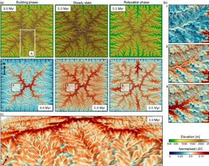
Figure 2.Outputs from the uniform precipitation (1 m yr−1) model.(a)The top row presents the evolution of the landscape at three time steps during the mountain-building phase (induced by a uniform uplift of 1 mm yr−1), just before the cessation of uplift at 5.0 Myr (landscape is at steady state, i.e. erosion balances uplift) and during the early phase of mountain collapse (5.5 Myr). The bottom row shows the spatial distributions of normalised LEC for the three considered time steps.(b)Detailed maps presenting changes in normalised LEC for regions 1, 2, and 3 defined in panel(a)and illustrating the geomorphic controls on LEC variability over time.(c)3-D view of the spatial patterns of the LEC index at 5 Myr with generally low LEC for valleys, minor peaks lower on the ridges, and high LEC on ridge flanks.
shows similar mid-elevation maximum LEC (i.e. peak of di-versity) over valley, catchment, and regional scales.
Our results show that under uniform tectonic and cli-matic forcing, landscape dynamics exert a 1st-order control on the landscape connectivity distribution, which is mostly distributed at mid-elevation and peaks on the highest flanks when geomorphic steady state is reached (Fig. 3a, thick blue line). The peak position is related to the symmetrical nature of the chosen boundary conditions and species niche width (σ =0.1) as shown in Sect. 4.1.
3.2 Orographic effect on patterns of landscape connectivity
To explore the influence of heterogenous precipitation on connectivity, we design a new set of experiments using a cou-pled climate and landscape evolution model in which precip-itation responds through space and time to the build-up of topography (i.e. orographic precipitation; Fig. 4a, b).
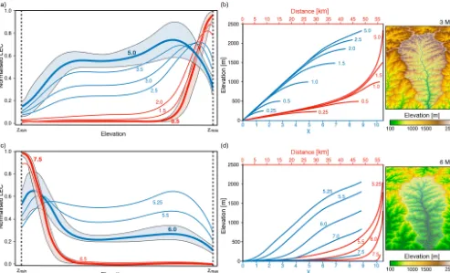
affect-Figure 3.Analysis of uniform precipitation results. Panels(a)and(b)relate to the mountain-building phase (0–5 Myr) and panels(c)and(d) to the relaxation phase (5–10 Myr). Plots in panels(a)and(c)illustrate the elevational gradients of normalised LEC over time (corresponding numbers in millions of years (Myr) for each line). Blue and red lines represent the average of normalised LEC within elevational bands. Blue and red areas are the standard deviation computed based on normalised LEC values as a function of site elevation at 5 and 6 Myr (blue areas) and 0.5 and 7.5 Myr (red areas). For plots(a)and(c), line colours reflect different stages of landscape evolution. In panel(a)the change from red to blue marks the disappearance of uplifted plateau. In panel(c)the change from blue to red relates to the erosion of 50 % of the maximum elevation obtained at steady state. These two plots have a moving horizontal scale aszminandzmaxchange with time. Panels(b) and(d)show main-stream temporal evolution for the catchment area (region A) defined in Fig. 2a and displayed at 3 and 6 Myr, respectively (right side). For the considered catchment, we show the extracted information from main channel profiles based onχplot analysis (Perron and Royden, 2013) (blue) and longitudinal river profiles (red) over time (associated time in millions of years (Myr) is given for each line).
ing river networks through reorganisation and concomitantly changing the topologies and geometries of drainage basins (Fig. 4e).
Similar to the uniform precipitation model, we observe a temporal migration of the LEC maximum from the uplifted plateau towards the bottom of the valleys. However, we find some specific features driven by the geomorphic responses to orographic precipitation (as shown by the LEC distribution at steady state between Figs. 2a and 4d) with a clear corre-lation between sites with high- or low-connectivity areas and windward- or leeward-facing catchments. It shows how up-lift and its effect on regional climate influence landscape con-nectivity with the development of geographic connections or barriers as topography changes.
The study of two specific catchments sharing a common drainage divide further highlights these effects. In Fig. 5, we note that both leeward and windward catchments exhibit similar hump-shaped patterns of LEC, indicative of
mid-elevation peaks, with higher connectivity on the windward-facing area compared to the leeward-windward-facing one. Tempo-ral evolution analysis through the complete orogenic cycle shows optimum landscape connectivity during the mountain-building phase at middle to high elevations as illustrated by the broader ranges of LEC values at 2.5 Myr compared to the ones at 5.5 Myr (Fig. 5b).
4 Discussion
bio-T. Salles et al.: Mapping landscape connectivity under tectonic and climatic forcing 901
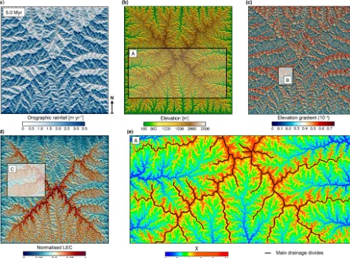
Figure 4.Generated outputs of the coupled landscape evolution and orographic precipitation models at the end of the uplift phase (5.0 Myr). (a)Induced rainfall map from the orographic model in which precipitation is determined by prevailing upslope winds (coming from the south) and by the moisture content of the air. Rainfall distribution is characterised by precipitation maxima on the windward face of the divides. (b)Resulting elevation grid for which the topographic evolution of the mountain ranges is affected by the spatial pattern of precipitation and tectonics. During the building phase, main drainage divides continuously migrate towards the drier side and asymmetric topography develops with steeper regions(c)on the leeward side of the ranges.(d)Resulting normalised LEC showing specific patterns of distribution with higher values obtained on windward-facing catchments. At this time step, lower LECs are generally found in valleys and mountain tops, and higher LECs are found on the flanks of both the mountain tops and main valley systems.(e)χmap (Perron and Royden, 2013; Willett et al., 2014) for inset A (shown in panelb) highlighting discontinuousχacross drainage divides, with largerχvalues on the leeward-facing catchments (victimbasins) compared to the windward ones (aggressorbasins). Insets B and C refer to the region used in the analysis performed in Figs. 5 and 9, respectively.
diversity using a similar metacommunity model as the one proposed in Bertuzzo et al. (2016) and discuss the possi-ble roles of geomorphological changes in patterns of species richness. By defining isolated regions as places with low con-nectivity, we then analyse how they evolve during simulated orogenic cycles.
4.1 Impact of forcing conditions and species niche width on connectivity mapping
In our experimental setting, we have deliberately chosen a simple model of an evolving landscape similar to existing
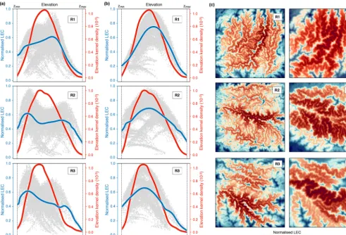
Figure 5.Temporal evolution of normalised LEC distribution patterns between windward (C1) and leeward (C2) catchments sharing a common divide (region B defined in Fig. 4c).(a)Normalised connectivity maps at 2.5 and 5.5 Myr; the white line represents the drainage-divide position at the current time step. The black dotted line shows the drainage-divide position at 2.5 Myr and black arrows its migration direction. Contour lines are defined every 250 m and range between 500 and 1750 m.(b)Plots of normalised LEC (grey dots), the average line of LEC within elevational bands (blue lines), and elevation kernel density (red lines) for the entire simulated domain at chosen time intervals. Normalised LEC for points belonging to the windward and leeward catchments (C1 and C2, respectively) are highlighted. The normalised LEC exhibits a typical pattern, with higher values and broader ranges during the mountain-building phase at middle to high elevations.
the simulated landscape is again purely erosional (similar to the homogeneous model proposed in Roy et al., 2015). Eval-uating how LEC will change for constructional landscapes (Craw et al., 2015, 2019) requires different tectonic condi-tions and is beyond the scope of this paper.
The general pattern of geomorphological evolution un-der uniform precipitation is presented in Fig. 6a for the first 5 Myr and corresponds to the mountain-building phase. As for the previous cases, the evolution of the experiment in-volves a growth phase followed by a steady-state phase (Bon-net and Crave, 2003; Castelltort and Yamato, 2013). Dur-ing the initial plateau uplift (e.g. growth phase), some topo-graphic incisions form along the western open border of the model. As uplift continues, these incisions grow and propa-gate inward until there is complete dissection of the plateau (third map on the right-hand side of Fig. 6a). The obtained fluvial landscapes display dendritic networks, and river
lon-gitudinal profiles present a concave upward shape character-istic of bedrock river systems (as for Fig. 3b).
T. Salles et al.: Mapping landscape connectivity under tectonic and climatic forcing 903
Figure 6.Outputs from the modified uniform precipitation model with only one fixed boundary along the western border of the simulated domain.(a)Maps of the evolution of the landscape at three time steps during the growth phase (induced by a uniform uplift of 1 mm yr−1). Panels(b)and(c)show the results obtained with two ratios forσ/(zmax−zmin) of 0.1 and 0.2, respectively. In both cases, we present on the left the average line of LEC within elevational bands (blue lines) and the elevation kernel density (red lines) for the entire simulated domain at steady state (5 Myr); on the right is the corresponding normalised connectivity map.
is less constrained by elevational barriers, and thus LEC is mostly controlled by the abundance of sites with similar el-evation in the simulated domain (i.e. the elel-evation frequency distribution as shown by the blue lines in Figs. 6c and 7b). Bertuzzo et al. (2016) show that for very largeσ, LEC
Figure 7.Connectivity results for the regions (R1, R2, and R3) presented in Fig. 6a. Panels(a)and(b)show the corresponding average line of LEC within elevational bands (blue lines) and the elevation kernel density (red lines) for two species niche width ratios of 0.1 and 0.2. Panel(c)presents the normalised connectivity map for the two width ratios and for the three regions.
4.2 LEC as a measure of biodiversity
Bertuzzo et al. (2016) have shown that when applied to real landscapes, the LEC metric predicts theαdiversity simulated by the full metacommunity model well. Here we perform a similar analysis on our simulated landscape and estimate for both scenarios (uniform and orographic rain) the correlations between LEC and simulated local species richness (α diver-sity).
To do so, we use a zero-sum metacommunity model (Hubbell, 2001) in which local communities (N) are defined on an regular 2-D elevation mesh. The zero-sum assumption states that each local community is saturated at all times, which means that the total number of individualsnin a par-ticular point is constant over time. In such a case and for any given time, the entire region is made of a population ofN·n
individuals, whereNis equivalent to the number of points on the grid. The population number is made of different species which have different elevational niches. Each of these niches describes the competitive ability of particular species with elevation and is defined with a Gaussian function following
Rybicki and Hanski (2013) (Bertuzzo et al., 2016):
fi(z)=fmaxie
−(z−zopti)2 2σ2
i , (7)
withfi(z) the competitive ability of species i at elevation
z. The elevation zopti is the optimal elevation for which the competitive ability equals fmaxi and σi is the niche width for speciesi as defined in Eq. (6). In addition to the zero-sum assumption, we suppose that all species have the same niche widthσi=σ and maximum competitive ability
fmaxi=fmaxas well as similar rates of dispersal, death, and fertility.
T. Salles et al.: Mapping landscape connectivity under tectonic and climatic forcing 905
is selected with a probability proportional to the values of
fi(z) for all the individuals living in the vicinity of the local community (wherezis the elevation of the considered local community). Second, the offspring is an individual belong-ing to a new species that does not already exist in the system. This second option is probabilistically selected at every time step and allows us to model both speciation and immigra-tion from external communities (Hubbell, 2001; Chave et al., 2002). When a competitor from a new species enters the sys-tem its optimal elevationzoptiis drawn from a uniform distri-bution spanning twice the relief of the system to avoid edge effects (Bertuzzo et al., 2016).
This metacommunity model is applied on the elevation grids obtained from our landscape evolution model. In all simulations, the system is initially populated by one single species and is run until a statistically steady state is reached (∼104generations, where a generation isN·ntime steps). As in Bertuzzo et al. (2016), we consider periodic boundary conditions. The parameter fmax does not affect the system dynamics and is, without loss of generality, set to 1.
Figure 8 presents the relationships between calculated LEC and local species richness for the simulated landscapes at steady state. Overall, we have Pearson’s correlations (R) of>70 %, which is considered to be relatively strong. These results are in agreement with the Bertuzzo et al. (2016) study and consolidate the idea that the LEC calculation is able to predict theαdiversity well, especially in the case of uniform rainfall. Therefore, if LEC captures the regional variability of community diversity, one can deduce from its distribution the temporal and spatial evolution of species richness.
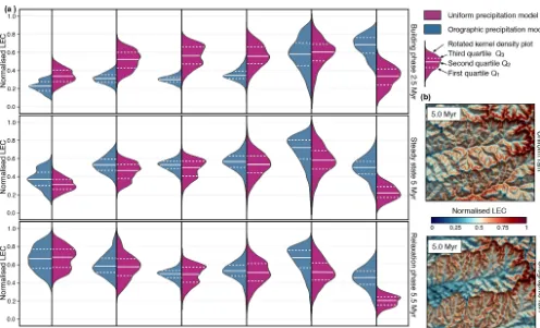
We provide in Fig. 9 a statistical summary of the LEC evolution for the two climatic scenarios. LEC predicts bio-diversity peaks when the landscape reaches a geomorpho-logical steady state, and maximum species richness is ob-served at mid-elevation (Fig. 9a – 0.7< z/zmax<0.9) as ob-served in nature (Grytnes and Vetaas, 2002; Colwell et al., 2004; Brehm et al., 2007). Interestingly, when using a coupled climate–landscape model, windward-facing regions host higher biodiversities. During relaxation phase, when tec-tonic forcing ceases, the peak in species richness shifts from middle to low elevations (bottom graph in Fig. 9a). From the figure, we infer that mapped areas showing strong connec-tivity values (i.e. high LEC) within a given elevational band have a direct effect on the biodiversity they host (Rahbek, 1997; McCain, 2007). We also hypothesise that these areas represent regions of high local species richness as local com-munities can be gathered from a more diverse regional pool of species that are fit to live at a similar elevation (Romdal and Grytnes, 2007).
In summary, LEC calculation can be used to estimate in a simple way the temporal and spatial evolution of biodiver-sity distribution induced by changes in landscape structure over geological time. Based on LEC distribution at steady state, we found that species richness in mountainous land-scapes reaches its peak at mid-elevation not only because
this is where the maximum surface area available to species is located, but also because species can move up or down to accommodate climate warming or cooling, respectively.
There are many biologic and abiotic properties that drive species richness in mountainous landscapes (Hoorn et al., 2010, 2013; Giezendanner et al., 2019). For example, moun-tains provide species with a rich variety of environmental conditions over restricted surface areas (e.g. range of temper-ature, solar irradiation, wind exposure, moisture and rainfall, soils thickness, and composition to cite a few). In this study, we have limited our exploration to the role of morphological changes imposed by uniform tectonic, riverine, and climatic processes, and we found that these changes alone could ex-plain to the 1st order the biodiversity found in mountainous regions.
4.3 Dynamics of geomorphically driven isolation
From the LEC values, one can derive geomorphically driven isolation by finding spatial regions of low LEC compared to their surrounding areas. Here, we apply an approach similar to a depression-filling algorithm (Barnes and Lehman, 2013) using the LEC values instead of the elevation. Isolated ar-eas in that sense represent depressions or inwardly draining regions of the LEC map which have no outlet. To prevent coalescence of these isolated regions (i.e. small depressions within bigger ones), one can apply a threshold on the filling limit of the LEC map. Increasing such a threshold produces a smaller number of isolated regions but with larger areas.
In Fig. 10, we evaluate through time these areas of low LEC values (normalised LEC below 20 %) and analyse series of metrics: mean LEC, mean area, and mean elevation. Our results show that the competition between mountain build-ing and erosion increases the number of isolated regions dur-ing the orogenic phase (Fig. 10a). Orographic precipitation fosters faster isolation than the uniform precipitation model (red line trends in Fig. 10a), especially on the steeper and drier leeward sides (rain shadow zones) of the drainage di-vides (Fig. 10b). For the uniform rain model, we observe a decrease in the average area of these isolated regions con-comitant with catchment stabilisation and the emergence of the steady state (light grey line in Fig. 10a). For both precip-itation scenarios, the cessation of tectonic activity at 5 Myr results in a rapid decrease in the number of isolated regions associated with an initial episode of augmentation of mean area that lasts no more than 250 000 years. We attribute this peculiar effect to the fast widening of valley high- and mid-elevation zones related to the adjustment of catchment mor-phology and induced by the advective slope retreat predom-inant across the valley heads (Pelletier, 2011). Hence, our model predicts an increase in isolation during the mountain-building phase and a decrease during the relaxation phase.
Figure 8.LEC versus local species richness (αdiversity) for simulated landscape at steady state (5 Myr) under uniform rainfall(a)and orographic precipitation(b). Theαdiversity patterns result from the zero-sum metacommunity model described below. Correlations between
αdiversity and LEC are presented (blue dots), as are regression and kernel density fits for each case. We also provide the resulting Pearson’s coefficients for correlation betweenαdiversity and LEC values.
Figure 9. Temporal and spatial statistical analysis of normalised LEC based on categorical elevation data (defined within six bands of
T. Salles et al.: Mapping landscape connectivity under tectonic and climatic forcing 907
Figure 10.Temporal evolution of the isolating effect of mountain geomorphology derived from LEC computation. The method consists of mapping and integrating over space and time regions of lower connectivities (normalised LEC <20 %) surrounded by higher ones. (a)Analysis of isolated regions for the uniform and orographic precipitation simulations. Each panel presents the mean elevation (zmean– dark grey), LEC (LECmean– black), and area (Amean– light grey) for the isolated regions as well as the total number of extracted regions (red line) through time.(b)Normalised connectivity maps showing for the orographic model the distribution of isolated regions (magenta areas) at three time intervals. The considered maps correspond to the highlighted region C defined in Fig. 4d. Both simulations exhibit a similar trend with an increase in the number of isolated regions during the building phase (shaded blue area) followed by a period of stabilisation and a rapid decrease during the relaxation phase (shaded red area). We note a sharp increase in mean area at 5 Myr attributed to the rapid adjustment of upper valley slopes following the cessation of uplift.
low LEC areas should potentially correspond to places where species get trapped into isolated refuges, and such ecological niches should favour speciation and endemism.
Not surprisingly, it has been found that the potential for isolation increases in more topographically diverse areas (Ali and Aitchison, 2014; Gillespie and Roderick, 2014). In re-cent years, several studies have shown that isolation induced by uplift and climatic processes plays a central part in shap-ing biodiversity (Wang et al., 2009; Craw et al., 2015), and the mapping of geomorphically driven low landscape con-nectivity could potentially highlight these areas of speciation hotspots. Therefore, the LEC calculation could provide an efficient way to identify and manage regions of higher con-servation value.
not distributed continuously over elevation gradients and the associated isolated regions will likely be found at different elevations. Therefore, the prediction of increasing endemism with higher elevation might not always be the rule.
5 Conclusions
This paper presents a methodology to quantify landscape connectivity under tectonic and climatic forcing. Over geo-logical timescales (millions of years), tectonics and surface processes conspire to transform flat regions into complex dissected mountainous landscapes. We used landscape ele-vational connectivity (LEC) to measure the connectivity be-tween sites of similar elevations (Bertuzzo et al., 2016). We show that this abiotic parameter is able to account for up to 80 % of the αdiversity predicted by a zero-sum metacom-munity model (Hubbell, 2001; Rybicki and Hanski, 2013), and therefore it could potentially explain the 1st-order distri-bution of biodiversity found in mountainous regions (Ali and Aitchison, 2014; Steinbauer et al., 2018). In the future, we can easily improve the predictive capacity of this metric by integrating fitness parameters other than elevation.
From the LEC calculation, one can quantify the role of geomorphology in landscape connectivity and topography-driven isolation. As the periodicity of isolation and connec-tion dictates evoluconnec-tionary outcomes, understanding this dy-namic might be used to test models of biological diversifi-cation and to understand species distribution and biodiver-sity patterns through time. Our results suggest that peaks in species richness for mountainous landscapes can be derived from the analysis of the dynamic organisation of geomorphic features as they evolved in response to tectonic, climatic, and erosion processes. These features might be inferred from physiographic metrics such asχmaps, in situ observations, river longitudinal profiles, or landscape evolution modelling. We also found that geomorphically driven isolation has the potential to increase rates of speciation over the entire ele-vational range. This is an important outcome that could po-tentially lead to the reassessment of the spatial viability of existing conservation sites and could help us improve future conservation planning, policy, and practice (Mokany et al., 2012).
Code and data availability. The results and data presented and discussed in this paper were simulated using theBadlandsmodel (https://badlands.readthedocs.io/en/latest/; Salles, 2016), and the connectivity maps were obtained from the bioLECPython pack-age (https://biolec.readthedocs.io/en/latest/; Salles and Rey, 2019). All the model outputs were visualised using the Python Matplotlib library for standard graphics, Seaborn data visualisation library for statistical graphics, and the Paraview software (v5.2.0; https: //www.paraview.org, last access: 27 September 2019) from Kit-ware, Sandia National Labs, and CSimSoft for 3-D graphics and 2-D maps.
Author contributions. TS developed the code, designed the ex-periment, and contributed to output analysis and paper writing; PR contributed to output analysis and interpretation, as well as paper writing; EB developed the code and contributed to output analysis, interpretation, and paper writing.
Competing interests. The authors declare that they have no con-flict of interest.
Acknowledgements. The authors acknowledge the Sydney In-formatics Hub and the University of Sydney’s high-performance computing cluster Artemis for providing the high-performance computing resources that contributed to the research results re-ported within this paper. We thank Phaedra Upton, the anonymous reviewer, and the journal editor for their comments that greatly im-proved the paper.
Review statement. This paper was edited by Robert Hilton and reviewed by Phaedra Upton and one anonymous referee.
References
Ali, J. R. and Aitchison, J. C.: Exploring the combined role of eustasy and oceanic island thermal subsidence in shaping biodiversity on the Galápagos, J. Biogeogr., 41, 1227–1241, https://doi.org/10.1111/jbi.12313, 2014.
Anders, A. M., Roe, G. H., Montgomery, D. R., and Hallet, B.: Influence of precipitation phase on the form of mountain ranges, Geology, 36, 479–482, https://doi.org/10.1130/G24821A.1, 2008.
Badgley, C.: Tectonics, topography, and mammalian diver-sity, Ecography, 33, 220–231, https://doi.org/10.1111/j.1600-0587.2010.06282.x, 2010.
Barnes, R. and Lehman, M.: Priority-Flood: An Optimal Depression-Filling and Watershed-Labeling Algorithm for Digital Elevation Models, Comput. Geosci., 62, 117–127, https://doi.org/10.1016/j.cageo.2013.04.024, 2013.
Bertuzzo, E., Rodriguez-Iturbe, I., and Rinaldo, A.: Metapopulation capacity of evolving fluvial landscapes, Water Resour. Res., 51, 2696–2706, https://doi.org/10.1002/2015WR016946, 2015. Bertuzzo, E., Carrara, F., Mari, L., Altermatt, F., Rodriguez-Iturbe,
I., and Rinaldo, A.: Geomorphic controls on elevational gradients of species richness, P. Natl. Acad. Sci. USA, 113, 1737–1742, https://doi.org/10.1073/pnas.1518922113, 2016.
Bonnet, S.: Shrinking and splitting of drainage basins in orogenic landscapes from the migration of the main drainage divide, Nat. Geosci., 2, 766–771, https://doi.org/10.1038/ngeo666, 2009. Bonnet, S. and Crave, A.: Landscape response to climate change:
Insights from experimental modeling and implications for tec-tonic versus climatic uplift of topography, Geology, 31, 123–126, 2003.
T. Salles et al.: Mapping landscape connectivity under tectonic and climatic forcing 909
Brown, J. H.: Why are there so many species in the tropics?, J. Bio-geogr., 41, 8–22, https://doi.org/10.1111/jbi.12228, 2014. Carrara, F., Altermatt, F., Rodriguez-Iturbe, I., and Rinaldo, A.:
Dendritic connectivity controls biodiversity patterns in experi-mental metacommunities, P. Natl. Acad. Sci. USA, 109, 5761– 5766, https://doi.org/10.1073/pnas.1119651109, 2012.
Castelltort, S. and Yamato, P.: The influence of surface slope on the shape of river basins: Comparison between nature and numerical landscape simulations, Geomorphology, 192, 71–79, https://doi.org/10.1016/j.geomorph.2013.03.022, 2013. Chave, J., Muller-Landau, H. C., and Levin, S. A.: Comparing
Clas-sical Community Models: Theoretical Consequences for Patterns of Diversity, Am. Nat., 159, 1–23, 2002.
Chen, A., Darbon, J., and Morel, J.-M.: Landscape evolution mod-els: a review of their fundamental equations, Geomorphology, 219, 68–86, 2014.
Colwell, R. K., Rahbek, C., and Gotelli, N. J.: The Mid-Domain Ef-fect and Species Richness Patterns: What Have We Learned So Far?, Am. Nat., 163, E1–E23, https://doi.org/10.1086/382056, 2004.
Craw, D., Upton, P., Burridge, C. P., Wallis, G. P., and Waters, J. M.: Rapid biological speciation driven by tec-tonic evolution in New Zealand, Nat. Geosci., 9, 140–144, https://doi.org/10.1038/ngeo2618, 2015.
Craw, D., King, T. M., McCulloch, G. A., Upton, P., and Wa-ters, J. M.: Biological evidence constraining river drainage evolution across a subduction-transcurrent plate boundary transition, New Zealand, Geomorphology, 336, 119–132, https://doi.org/10.1016/j.geomorph.2019.03.032, 2019. Dietrich, W. E., Reiss, R., Hsu, M. L., and Montgomery, D. R.: A
process-based model for colluvial soil depth and shallow lands-liding using digital elevation data, Hydrol. Process., 9, 383–400, 1995.
Dijkstra, E. W.: A note on two problems in connexion with graphs, Numer. Math., 1, 269–271, https://doi.org/10.1007/BF01386390, 1959.
Economo, E. P. and Keitt, T. H.: Network isolation and local di-versity in neutral metacommunities, Oikos, 119, 1355–1363, https://doi.org/10.1111/j.1600-0706.2010.18272.x, 2010. Elsen, P. R. and Tingley, M. W.: Global mountain topography and
the fate of montane species under climate change, Nat. Clim. Change, 5, 772–776, https://doi.org/10.1038/nclimate2656, 2015.
Emerson, B. C. and Kolm, N.: Species diversity can drive spe-ciation, Nature, 434, 1015, https://doi.org/10.1038/nature03450, 2005.
Ferrier, K. L., Huppert, K. L., and Perron, J. T.: Climatic control of bedrock river incision, Nature, 496, 206–209, https://doi.org/10.1038/nature11982, 2013.
Giezendanner, J., Bertuzzo, E., Pasetto, D., Guisan, A., and Rinaldo, A.: A minimalist model of extinction and range dynamics of virtual mountain species driven by warming temperatures, PLoS ONE, 14, e0213775, https://doi.org/10.1371/journal.pone.0213775, 2019.
Gillespie, R. G. and Roderick, G. K.: Geology and cli-mate drive diversification, Nature, 509, 297–298, https://doi.org/10.1038/509297a, 2014.
Grytnes, J. A. and Vetaas, O. R.: Species Richness and Altitude: A Comparison between Null Models and Interpolated Plant Species
Richness along the Himalayan Altitudinal Gradient, Nepal, Am. Nat., 159, 294–304, https://doi.org/10.1086/338542, 2002. Hoorn, C., Wesselingh, F. P., ter Steege, H., Bermudez, M. A.,
Mora, A., Sevink, J., Sanmartín, I., Sanchez-Meseguer, A., An-derson, C. L., Figueiredo, J. P., Jaramillo, C., Riff, D., Negri, F. R., Hooghiemstra, H., Lundberg, J., Stadler, T., Särkinen, T., and Antonelli, A.: Amazonia Through Time: Andean Uplift, Cli-mate Change, Landscape Evolution, and Biodiversity, Science, 330, 927–931, https://doi.org/10.1126/science.1194585, 2010. Hoorn, C., Mosbrugger, V., Mulch, A., and Antonelli, A.:
Biodiversity from mountain building, Nat. Geosci., 6, 154, https://doi.org/10.1038/ngeo1742, 2013.
Hubbell, S. P.: The Unified Neutral Theory of Biodiversity and Biogeography (MPB-32), Princeton University Press, Princeton, New Jersey, 2001.
Kearney, M. and Porter, W.: Mechanistic niche modelling: com-bining physiological and spatial data to predict species’ ranges, Ecol. Lett., 12, 334–350, https://doi.org/10.1111/j.1461-0248.2008.01277.x, 2009.
Kessler, M., Kluge, J., Hemp, A., and Ohlemüller, R.: A global comparative analysis of elevational species richness patterns of ferns, Global Ecol. Biogeogr., 20, 868–880, https://doi.org/10.1111/j.1466-8238.2011.00653.x, 2011. Liu, C., Dudley, K. L., Xu, Z.-H., and Economo, E. P.:
Moun-tain metacommunities: climate and spatial connectivity shape ant diversity in a complex landscape, Ecography, 41, 101–112, https://doi.org/10.1111/ecog.03067, 2018.
Lomolino, M. V.: Elevation gradients of species-density: histori-cal and prospective views, Global Ecol. Biogeogr., 10, 3–13, https://doi.org/10.1046/j.1466-822x.2001.00229.x, 2001. MacArthur, R. H. and Wilson, E. O.: The Theory of Island
Biogeog-raphy, Princeton University Press, Princeton, New Jersey, 1967. Martensen, A., Saura, S., and Fortin, M.-J.: Spatio-temporal
connectivity: assessing the amount of reachable habitat in dynamic landscapes, Methods Ecol. Evol., 8, 1253–1264, https://doi.org/10.1111/2041-210X.12799, 2017.
McCain, C. M.: Area and mammalian elevation diver-sity, Ecology, 88, 76–86, https://doi.org/10.1890/0012-9658(2007)88[76:AAMED]2.0.CO;2, 2007.
McCain, C. M. and Grytnes, J.-A.: Elevational Gradi-ents in Species Richness, American Cancer Society, https://doi.org/10.1002/9780470015902.a0022548, 2010. Mokany, K., Harwood, T. D., Williams, K. J., and Ferrier, S.:
Dynamic macroecology and the future for biodiversity, Glob. Change Biol., 18, 3149–3159, https://doi.org/10.1111/j.1365-2486.2012.02760.x, 2012.
Mudd, S. M., Attal, M., Milodowski, D. T., Grieve, S. W. D., and Valters, D. A.: A statistical framework to quantify spa-tial variation in channel gradients using the integral method of channel profile analysis, J. Geophys. Res.-Earth, 119, 138–152, https://doi.org/10.1002/2013JF002981, 2014.
Muneepeerakul, R., Bertuzzo, E., Rinaldo, A., and Rodriguez-Iturbe, I.: Evolving biodiversity patterns in chang-ing river networks, J. Theor. Biol., 462, 418–424, https://doi.org/10.1016/j.jtbi.2018.11.021, 2019.
Perron, J. T. and Royden, L.: An integral approach to bedrock river profile analysis, Earth Surf. Proc. Land., 38, 570–576, https://doi.org/10.1002/esp.3302, 2013.
Rahbek, C.: The elevational gradient of species rich-ness: a uniform pattern?, Ecography, 18, 200–205, https://doi.org/10.1111/j.1600-0587.1995.tb00341.x, 1995. Rahbek, C.: The Relationship among Area, Elevation, and Regional
Species Richness in Neotropical Birds, Am. Nat., 149, 875–902, https://doi.org/10.1086/286028, 1997.
Rahbek, C.: The role of spatial scale and the perception of large-scale species-richness patterns, Ecol. Lett., 8, 224–239, https://doi.org/10.1111/j.1461-0248.2004.00701.x, 2005. Roe, G. H., Montgomery, D. R., and Hallet, B.: Orographic
precip-itation and the relief of mountain ranges, J. Geophys. Res.-Sol. Ea., 108, 2315, https://doi.org/10.1029/2001JB001521, 2003. Romdal, T. S. and Grytnes, J.: An indirect area effect on
el-evational species richness patterns, Ecography, 30, 440–448, https://doi.org/10.1111/j.0906-7590.2007.04954.x, 2007. Roy, S. G., Koons, P. O., Upton, P., and Tucker, G. E.: The
influence of crustal strength fields on the patterns and rates of fluvial incision, J. Geophys. Res.-Earth, 120, 275–299, https://doi.org/10.1002/2014JF003281, 2015.
Rybicki, J. and Hanski, I.: Species–area relationships and extinc-tions caused by habitat loss and fragmentation, Ecology Letters, 16, 27–38, https://doi.org/10.1111/ele.12065, 2013.
Salles, T.: Badlands: A parallel basin and land-scape dynamics model, SoftwareX, 5, 195–202, https://doi.org/10.1016/j.softx.2016.08.005, 2016 (model available at: https://badlands.readthedocs.io/en/latest/, last access: 27 September 2019).
Salles, T. and Hardiman, L.: Badlands: An open-source, flexible and parallel framework to study landscape dynamics, Comp. Geosci., 91, 77–89, 2016.
Salles, T. and Rey, P.: bioLEC: A Python package to measure Land-scape Elevational Connectivity, Journal of Open Source Soft-ware, 4, 1498, https://doi.org/10.21105/joss.01530, 2019 (code available at: https://biolec.readthedocs.io/en/latest/, last access: 27 September 2019).
Salles, T., Ding, X., and Brocard, G.: pyBadlands: A framework to simulate sediment transport, landscape dynamics and basin stratigraphic evolution through space and time, PLOS ONE, 13, 1–24, https://doi.org/10.1371/journal.pone.0195557, 2018a. Salles, T., Ding, X., Webster, J. M., Vila-Concejo, A.,
Bro-card, G., and Pall, J.: A unified framework for modelling sediment fate from source to sink and its interactions with reef systems over geological times, Sci. Rep., 8, 5252, https://doi.org/10.1038/s41598-018-23519-8, 2018b.
Smith, B. T., McCormack, J. E., Cuervo, A. M., Hickerson, M. J., Aleixo, A., Cadena, C. D., Pérez-Emán, J., Burney, C. W., Xie, X., Harvey, M. G., Faircloth, B. C., Glenn, T. C., Derryberry, E. P., Prejean, J., Fields, S., and Brumfield, R. T.: The drivers of tropical speciation, Nature, 515, 406–409, https://doi.org/10.1038/nature13687, 2014.
Smith, R. B. and Barstad, I.: A Linear Theory of Orographic Pre-cipitation, J. Atmos. Sci., 61, 1377–1391, 2004.
Solé, R. V. and Bascompte, J.: Self-Organization in Complex Ecosystems (MPB-42), Princeton University Press, Princeton, New Jersey, 2006.
Steinbauer, M. J., Field, R., Grytnes, J., Trigas, P., Ah-Peng, C., Attorre, F., Birks, H. J. B., Borges, P. A. V., Cardoso, P., Chou, C., Sanctis, M. D., de Sequeira, M. M., Duarte, M. C., Elias, R. B., Fernández-Palacios, J. M., Gabriel, R., Gereau, R. E., Gillespie, R. G., Greimler, J., Harter, D. E. V., Huang, T., Irl, S. D. H., Jeanmonod, D., Jentsch, A., Jump, A. S., Kueffer, C., Nogué, S., Otto, R., Price, J., Romeiras, M. M., Strasberg, D., Stuessy, T., Svenning, J., Vetaas, O. R., Beierkuhnlein, C., and Gillespie, T.: Topography-driven isolation, speciation and a global increase of endemism with elevation, Global Ecol. Biogeogr., 25, 1097– 1107, https://doi.org/10.1111/geb.12469, 2016.
Steinbauer, M. J., Grytnes, J.-A., Jurasinski, G., Kulonen, A., Lenoir, J., Pauli, H., Rixen, C., Winkler, M., Bardy-Durchhalter, M., Barni, E., Bjorkman, A. D., Breiner, F. T., Burg, S., Czortek, P., Dawes, M. A., Delimat, A., Dullinger, S., Erschbamer, B., Felde, V. A., Fernández-Arberas, O., Fossheim, K. F., Gómez-García, D., Georges, D., Grindrud, E. T., Haider, S., Haugum, S. V., Henriksen, H., Herreros, M. J., Jaroszewicz, B., Jaroszyn-ska, F., Kanka, R., Kapfer, J., Klanderud, K., Kühn, I., Lam-precht, A., Matteodo, M., di Cella, U. M., Normand, S., Od-land, A., Olsen, S. L., Palacio, S., Petey, M., Piscová, V., Sed-lakova, B., Steinbauer, K., Stöckli, V., Svenning, J.-C., Teppa, G., Theurillat, J.-P., Vittoz, P., Woodin, S. J., Zimmermann, N. E., and Wipf, S.: Accelerated increase in plant species richness on mountain summits is linked to warming, Nature, 556, 231–234, https://doi.org/10.1038/s41586-018-0005-6, 2018.
Tischendorf, L. and Fahrig, L.: On the usage and mea-surement of landscape connectivity, Oikos, 90, 7–19, https://doi.org/10.1034/j.1600-0706.2000.900102.x, 2000. Tucker, G. and Hancock, G. R.: Modelling landscape evolution.,
Earth Surf. Proc. Land., 35, 28–50, 2010.
van der Walt, S., Schonberger, J., Nunez-Iglesias, J., Boulogne, F., Warner, J., Yager, N., Gouillart, E., and Yu, T.: Scikit Image Con-tributors – scikit-image: image processing in Python, PeerJ, 2, e453, https://doi.org/10.7717/peerj.453, 2014.
Wallace, A. R.: On the Zoological Geography of the Malay Archipelago, Journal of the Proceedings of the Linnean Society of London. Zoology, 4, 172–184, https://doi.org/10.1111/j.1096-3642.1860.tb00090.x, 1860.
Wang, I. J., Savage, W. K., and Shaffer, H. B.: Landscape genetics and least-cost path analysis reveal unexpected dispersal routes in the California tiger salamander (Ambystoma californiense), Mol. Ecol., 18, 1365–1374, https://doi.org/10.1111/j.1365-294X.2009.04122.x, 2009.
Whipple, K. and Tucker, G.: Dynamics of the stream-power river in-cision model: implications for height limits of mountain ranges, landscape response timescales, and research needs, J. Geophys. Res., 104, 17661–17674, 1999.
Whipple, K. X., Forte, A. M., DiBiase, R. A., Gasparini, N. M., and Ouimet, W. B.: Timescales of landscape response to divide mi-gration and drainage capture: Implications for the role of divide mobility in landscape evolution, J. Geophys. Res.-Earth, 122, 248–273, https://doi.org/10.1002/2016JF003973, 2016. Willett, S. D., McCoy, S. W., Perron, J. T., Goren, L., and Chen,