TRIANGULAR FUZZY MULTINOMIAL CONTROL CHART WITH VARIABLE SAMPLE SIZE USING – CUTS

TRIANGULAR FUZZY MULTINOMIAL

CONTROL CHART WITH VARIABLE

SAMPLE SIZE USING

α

– CUTS

S.Selva Arul Pandian Assistant Professor (Sr.) in Statistics,

Department of Mathematics,

K.S.R College of Engineering, Tiruchengode – 637 215. Tamil Nadu, India. E-Mail Id: [email protected].,

Dr.P.Puthiyanayagam

Professor and Controller of Examination, Department of Statistics,

Subbalakshmi Lakshmipathy College of Science, Madurai - 625 022, Tamil Nadu, India.

Abstract:

Statistical Process Control concepts and methods have been very important in the manufacturing and process industries. The main objective is to monitor the performance of a process over time in order for the process to achieve a state of statistical control. So many of the quality characteristics found in these process industries are not easily measured on a numerical scale. Quality characteristics of this type are called attribute data. Many basic attribute control charts like, p-chart, c-chart and u-chart are readily available in this process industry. This paper designs control chart for multiple-attribute quality characteristics. Aggregate sample quality is estimated by using interactive weighted addition of fuzzy values assigned to each quality characteristics. Triangular Fuzzy multinomial Control charts are drawn using Multinomial distribution using α – cuts for variable sample sizes. The proposed method is compared and numerical example is the evidence for improvement in the process.

Keyword: TFM chart, Multi-attribute chart, α – cuts chart, Multinomial chart, Fuzzy control chart

1. Introduction:

Statistical Process control (SPC) represents a set of tools for managing process, and also for determining and monitoring the quality of final product within an organization. The SPC can be viewed as a strategy for reducing variation in production process, where the variation represents an unwanted thing for any company producing goods or providing service. D.C. Montgomerry [9] illustrated as “Statistical Process control is a powerful collection of problem - solving tools useful in achieving process stability and improving capability through the reduction of variability. In 1924, Walter Shewhart designed the first control charts as follows: Let w be a number of samples used to measure some quality characteristic of interest and suppose that the mean of w is

μ

w and the standard deviation of w is



w. Then the upper control limit, central limit and lower control

limit are respectively given by

UCL =

μ

w +

k

σ

w , CL =

μ

w, LCL =

μ

w 

k

σ

w

Where k is the “distance” of the control limits from the centre line and it is expressed in unit’s standard deviation.

A single measureable quality characteristic such as dimension, weight or volume is called a variable. In such cases, control charts for variables are used. These include - chart for controlling the process average and R-chart for controlling the process variability. If the quality related characteristics such as characteristics for appearance, softness, colour, taste, etc., attribute control chart such as p-chart , c-chart are used to monitor the production process. Sometimes classified as either “conforming or nonconforming”, depending upon whether or not they must meet the specifications. The p-chart

2.

Fuzzy logic and Linguistic Variable:

average, fuzzy mode, and fuzzy median and α- level fuzzy-midrange, to construct the control chart. The membership functions defined for the linguistic variables in the above method are chosen arbitrarily and hence decision for process control may change as per the user’s choice of values of decision parameter. Amirzadeh et al. [1] have developed Fuzzy Multinomial control chart for fixed Sample Size and Pandurnagan et al. [11] illustrated fuzzy multinomial control chart based on linguistic variable which is classified into more than two categories with variable sample size.

In this paper, a Triangular Fuzzy Multinomial control chart (TFM chart) with VSS for linguistics variables using fuzzy number with α –cut fuzzy midrange transform techniques is proposed. The proposed method is compared with regular p-chart and FM-chat with VSS and which is more effective.

3. Methodology:

Based up on fuzzy set theory, a linguistics variable which is classified by the set of k mutually, exclusive members 1, 2, … . . . We estimate the weight to each term li and the fuzzy set is defined as

1, 1 , 2 , 2 , … … , (1)

To monitor the out of control signal in the production process we are taking independent samples of different size and categorized as ‘perfect’, ‘good’, ‘poor’ etc form the {n1, n2, n3, …..ns).

4. Fuzzy Multinomial control chart:

Pandurnagan et al. [11], defined is a linguistic variable which can take k mutually exclusive members 1, 2, … . . and pi is the probability that an item li is produced. Then 1, 2, … . . has multinomial distribution with parameters nrand p1, p2, ….pk. It is known that each XiMarginally has Binomial distribution with parameters nr pi and nr pi (1- pi ) respectively. Then the FM Control Chart with VSS is given by

5. Triangular Fuzzy Multinomial control Chart:

is a linguistic variable which can categorize k mutually exclusive members 1, 2, … . . and each members are more skewed for each variable sample sizes. The weights of the membership degree are also assumed as 1, 0.75, 0.5, 0.25 and 0 in the Fuzzy Multinomial distribution control chart. To overcome these drawbacks, we propose Triangular Fuzzy multinomial Control chart with variable sample size based on α –cut fuzzy midrange transform techniques.

6. Fuzzy number construction:

A method of constructing fuzzy numbers is given in the following steps.

Step1: Let the observation for quality characteristics from samples of different sizes are assigned on a rank of

1 to k. a relative distance matrix D = [dij]kxk where dij = is evaluated.

Step 2: The average of relative distance for each li is calculate by . This distance average is

used to measure the centre of all the ranking for each quality characteristics.

Step3: Find a pair-wise comparison matrix P = [pij]kxk, where .

Step4: Evaluates weights by weight determination method of Saaty (1980) as ; 1, 2, …

where ∑ 1

Step5: The importance of degree wi represents the weight to be associated with li when estimating the mode of

the fuzzy number. The fuzzy mode is given by ∑

Step6: Separate the sample quality characteristics li and find as fuzzy subset A and C, which is by obtained by

and . The fuzzy subset A and C which is represented as follows

, , … . ,

And , , , , … . , ,

: Apply fuzzy multinomial distribution separately for the fuzzy subset A , M and C and find

∑ ∑ ∑

Step8: Apply an α – cut to the fuzzy sets, the values are obtained as follows

Step9: Construct -cut Triangular FM control chart based on Multinomial distribution

3 ,

3 ,

3

, ,

3 ,

3 ,

3

Where

Step10: α – level fuzzy midrange is one of four transformation techniques used to determine the fuzzy control

limits. These control limits are used to give a decision such as in-control or out-of-control for a process. In this study α – level fuzzy midrange is used as the fuzzy transformation method while calculating the control limits.

3

2

3

2

Step11: The definition of α- level fuzzy midrange for sample ni for Triangular FM control chart is defined

Step12: Then the condition of process control for each sample can be defined by as

7. Numerical Example:

The numerical example given by Pandurnagan et al. [11], are taken for constructing TFM control chart. On a production line, a visual control of the aluminum die-cast of a lighting component might have the following assessment possibilities

1.”reject” if the aluminum die-cast does not works;

2. ”poor quality” if the aluminum die-cast works but has some defects;

3. ”medium quality” if the aluminum die-cast works and has no defects, but has some aesthetic flaws; 4. “good quality” if the aluminum die-cast works and has no defects, but has few aesthetic flaws;

Table – 1.

7.1.

Construction of control limits for p-chart:

The value of can be calculated to the following ways

∑ ₁

∑

∑

, , , …

12 1 10 0.75 12 0.5 54 0.25 12 0

100 0.390

8 1 7 0.75 9 0.5 48 0.25 8 0

80 0.372

And so on, and the value of , the control limits for P-charts can be calculated as follows

, , , …

P D 0.120, P D 0.100, P D 0.075 ; and so on.

The control limits for P – chart is obtained as follows

∑

∑ 0.096

For sample 1: 0.096 3 . . 0.184

0.096

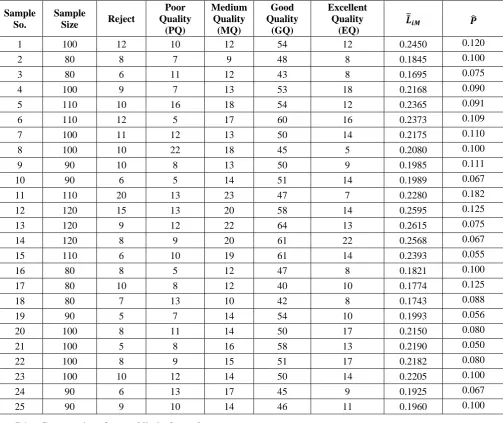
Sample So.

Sample

Size Reject

Poor Quality

(PQ)

Medium Quality

(MQ)

Good Quality

(GQ)

Excellent Quality

(EQ)

1 100 12 10 12 54 12 0.2450 0.120

2 80 8 7 9 48 8 0.1845 0.100

3 80 6 11 12 43 8 0.1695 0.075

4 100 9 7 13 53 18 0.2168 0.090

5 110 10 16 18 54 12 0.2365 0.091

6 110 12 5 17 60 16 0.2373 0.109

7 100 11 12 13 50 14 0.2175 0.110

8 100 10 22 18 45 5 0.2080 0.100

9 90 10 8 13 50 9 0.1985 0.111

10 90 6 5 14 51 14 0.1989 0.067

11 110 20 13 23 47 7 0.2280 0.182

12 120 15 13 20 58 14 0.2595 0.125

13 120 9 12 22 64 13 0.2615 0.075

14 120 8 9 20 61 22 0.2568 0.067

15 110 6 10 19 61 14 0.2393 0.055

16 80 8 5 12 47 8 0.1821 0.100

17 80 10 8 12 40 10 0.1774 0.125

18 80 7 13 10 42 8 0.1743 0.088

19 90 5 7 14 54 10 0.1993 0.056

20 100 8 11 14 50 17 0.2150 0.080

21 100 5 8 16 58 13 0.2190 0.050

22 100 8 9 15 51 17 0.2182 0.080

23 100 10 12 14 50 14 0.2205 0.100

24 90 6 13 17 45 9 0.1925 0.067

0.096 3 . . 0.008

For sample 2: 0.096 3 . . 0.195

0.096

0.096 3 . . 0.003 and so on.

7.2. Construction of control limits for FM-chart:

To construct the FM-chart, the control limits are computed for each sample as follows.

For sample 1: 3 0.375 3 √0.0008214 0.4609

∑ 0.3750

3 0.375 3 √0.0008214 0.2891

For sample 2: 3 0.3863 3 √0.001234 0.4917

∑ 0.3863

3 0.3863 3 √0.001234 0.2809 and so on.

Where ∑ and ∑ 1 2 ∑ ∑

7.3.

Construction of control limits for TFM-chart (Proposed Method):

To construct TFM control chart with VSS for each sample, first we must estimate

, for each Fuzzy subset as follows

For sample 1 ∑ 0.3063

∑ 0.2450

∑ 0.1688

For Sample 2 ∑ 0.3030

∑ 0.1855

∑ 0.1579 and so on.

Apply an α – cut to the fuzzy sets by taking α = 0.65, the values are obtained as follows

and

For sample 1

.

0.65

. 0.3069 0.65 0.2450 0.3063 0.2664

.

0.65

. 0.1688 0.65 0.1688 0.2450 0.2183

For sample 2 . 0.65

. 0.3030 0.65 0.1855 0.3030 0.2259

.

0.65

α – level fuzzy midrange is used as the fuzzy transformation method while calculating the control limits.

For Sample 1

. . 3

. .

. 0.2424 3 √ . . 0.2707

. .

.

. _{. .}

0.2424

. _{0.2424 3} √ . . _0.2141

For Sample 2

. . 3

. .

0.2190

. .

.

. _{. .}

0.2006

. 0.2006 3 √ . . 0.1758 and so on

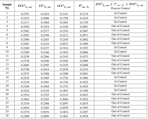
The Triangular Fuzzy Multinomial control chart for VSS with α – level fuzzy midrange for each samples are calculated and given in the table 2.

Table -2

Sample No

1 0.2664 0.2450 0.2183 0.00012552 0.00008 0.00005265

2 0.2259 0.1845 0.1752 0.00011592 0.00003 0.00001987

3 0.2269 0.1695 0.1539 0.00009359 0.00001 0.00000703

4 0.2836 0.2168 0.1873 0.00007422 0.00002 0.00001114

5 0.2788 0.2365 0.1967 0.00006538 0.00002 0.00001042

6 0.2777 0.2373 0.2019 0.00006567 0.00002 0.00001040

7 0.2754 0.2175 0.1851 0.00007553 0.00002 0.00001109

8 0.2693 0.2080 0.1746 0.00006192 0.00002 0.00001193

9 0.2477 0.1985 0.1776 0.00008933 0.00002 0.00001169

10 0.2517 0.1989 0.1815 0.00008859 0.00003 0.00002171

11 0.2876 0.2280 0.1856 0.00005528 0.00002 0.00001083

12 0.2970 0.2595 0.2110 0.00006092 0.00001 0.00000923

13 0.2843 0.2615 0.2166 0.00006297 0.00001 0.00000893

14 0.3115 0.2568 0.2114 0.00005899 0.00002 0.00000986

15 0.2735 0.2393 0.2040 0.00006809 0.00002 0.00001004

16 0.2245 0.1821 0.1725 0.00010790 0.00003 0.00002013

17 0.2349 0.1774 0.1613 0.00010200 0.00003 0.00002212

18 0.2337 0.1743 0.1592 0.00009504 0.00002 0.00001374

19 0.2401 0.1993 0.1820 0.00008958 0.00002 0.00001159

20 0.2816 0.2150 0.1835 0.00007175 0.00002 0.00001138

21 0.2594 0.2190 0.1931 0.00007701 0.00002 0.00001098

22 0.2727 0.2182 0.1888 0.00007859 0.00003 0.00001965

23 0.2670 0.2205 0.1894 0.00008123 0.00003 0.00001857

24 0.2464 0.1925 0.1689 0.00007779 0.00002 0.00001275

Evaluated weights by weight determination method of Saaty (1980) as where ∑ 1 are presented in table 3 through column from 7 to 11 and various probabilities corresponding to each sample are presented in the table 3 through column from 12 to 16.

Table 3

Samp

le No. Rej.

P Q

M

Q GQ

E

Q w1 w2 w3 w4 w5 p1 p2 p3 p4 p5

1 12 10 12 54 12 0.125 0.313 0.125 0.313 0.125 0.120 0.100 0.120 0.540 0.120

2 8 7 9 48 8 0.145 0.263 0.184 0.263 0.145 0.100 0.088 0.113 0.600 0.100

3 6 11 12 43 8 0.233 0.209 0.163 0.233 0.163 0.075 0.138 0.150 0.538 0.100

4 9 7 13 53 18 0.175 0.250 0.150 0.250 0.175 0.090 0.070 0.130 0.530 0.180

5 10 16 18 54 12 0.250 0.150 0.175 0.250 0.175 0.091 0.145 0.164 0.491 0.109

6 12 5 17 60 16 0.175 0.250 0.175 0.250 0.150 0.109 0.045 0.155 0.545 0.145

7 11 12 13 50 14 0.250 0.175 0.150 0.250 0.175 0.110 0.120 0.130 0.500 0.140

8 10 22 18 45 5 0.175 0.175 0.150 0.250 0.250 0.100 0.220 0.180 0.450 0.050

9 10 8 13 50 9 0.150 0.250 0.175 0.250 0.175 0.111 0.089 0.144 0.556 0.100

10 6 5 14 51 14 0.184 0.263 0.145 0.263 0.145 0.067 0.056 0.156 0.567 0.156

11 20 13 23 47 7 0.150 0.175 0.175 0.250 0.250 0.182 0.118 0.209 0.427 0.064

12 15 13 20 58 14 0.150 0.250 0.175 0.250 0.175 0.125 0.108 0.167 0.483 0.117

13 9 12 22 64 13 0.250 0.175 0.175 0.250 0.150 0.075 0.100 0.183 0.533 0.108

14 8 9 20 61 22 0.250 0.175 0.150 0.250 0.175 0.067 0.075 0.167 0.508 0.183

15 6 10 19 61 14 0.250 0.175 0.175 0.250 0.150 0.055 0.091 0.173 0.555 0.127

16 8 5 12 47 8 0.145 0.263 0.184 0.263 0.145 0.100 0.063 0.150 0.588 0.100

17 10 8 12 40 10 0.145 0.263 0.184 0.263 0.145 0.125 0.100 0.150 0.500 0.125

18 7 13 10 42 8 0.250 0.175 0.150 0.250 0.175 0.088 0.163 0.125 0.525 0.100

19 5 7 14 54 10 0.250 0.175 0.175 0.250 0.150 0.056 0.078 0.156 0.600 0.111

20 8 11 14 50 17 0.250 0.175 0.150 0.250 0.175 0.080 0.110 0.140 0.500 0.170

21 5 8 16 58 13 0.250 0.175 0.175 0.250 0.150 0.050 0.080 0.160 0.580 0.130

22 8 9 15 51 17 0.263 0.184 0.145 0.263 0.145 0.080 0.090 0.150 0.510 0.170

23 10 12 14 50 14 0.263 0.184 0.145 0.263 0.145 0.100 0.120 0.140 0.500 0.140

24 6 13 17 45 9 0.250 0.150 0.175 0.250 0.175 0.067 0.144 0.189 0.500 0.100

25 9 10 14 46 11 0.250 0.175 0.175 0.250 0.150 0.100 0.111 0.156 0.511 0.122

Table 4

Sample No

Process Control

1 _{0.2707 0.2424 0.2141 0.2176} In Control

2 _{0.2253 0.2006 0.1758 0.1919} In Control

3 _{0.2117 0.1904 0.1691 0.1759} In Control

4 _{0.2550 0.2354 0.2158 0.2081} Out-of-Control

5 _{0.2562 0.2377 0.2193 0.2007} Out-of-Control

6 _{0.2583 0.2398 0.2213 0.2071} Out-of-Control

7 _{0.2500 0.2303 0.2105 0.2002} Out-of-Control

8 _{0.2401 0.2219 0.2037 0.1909} Out-of-Control

9 _{0.2340 0.2127 0.1914 0.1933} In Control

10 _{0.2389 0.2166 0.1943 0.2004} In Control

11 _{0.2538 0.2366 0.2193 0.1972} Out-of-Control

12 _{0.2718 0.2540 0.2362 0.2089} Out-of-Control

13 _{0.2685 0.2505 0.2325 0.2088} Out-of-Control

14 _{0.2790 0.2614 0.2438 0.2193} Out-of-Control

15 _{0.2575 0.2388 0.2200 0.2061} Out-of-Control

16 _{0.2225 0.1985 0.1745 0.1896} In Control

17 _{0.2218 0.1981 0.1745 0.1832} In Control

18 _{0.2186 0.1964 0.1743 0.1825} In Control

19 _{0.2324 0.2110 0.1897 0.1950} In Control

20 _{0.2519 0.2325 0.2132 0.2033} Out-of-Control

21 _{0.2462 0.2263 0.2064 0.2022} Out-of-Control

22 _{0.2518 0.2308 0.2097 0.2035} Out-of-Control

23 _{0.2494 0.2282 0.2070 0.1993} Out-of-Control

24 _{0.2278 0.2076 0.1874 0.1857} Out-of-Control

25 _{0.2308 0.2099 0.1891 0.1878} Out-of-Control

From the above table, the process is out of control at samples at sample 4, the corresponding sample sizes are 100. The corresponding control limits are given by

For sample 4:

UCL = 0.2550 CL = 0.2354 LCL = 0.2158 0.2081 Sample Size 100

PR = 0.090 PPQ = 0.070 PMQ = 0.130 PGQ = 0.530 PEQ = 0.180 For Sample 5:

UCL = 0.2562 CL = 0.2377 LCL = 0.2193 0.2007 Sample Size 110

PR = 0.091 PPQ = 0.145 PMQ = 0.164 PGQ = 0.491 PEQ = 0.109 and so on.

I

t is clear that the TFM chart for VSS with α – level fuzzy midrange gives the first signal of special causes corresponding to 4th sample. The FM chart for VSS show the existence of assignable cause at 8th sample and in p-chart the first signal for out of control is identified at the 11th sample. Only 360 samples are inspected to get the first out of control signal, but the 780 and 1070 samples are to be inspected to get the alarm with the help of FM chart with VSS and p-chart respectively. TFM chart for VSS with α – level fuzzy midrange is more economical and more sensitive to identify the shift in the multi-attribute quality data.

8. Conclusion:

9. References:

[1] Amirzadeh.V., M.Mashinchi., M.A.Yagoobi. (2008). Construction of control chars using Fuzzy Multinomial Quality. Journal of Mathematics and Statistics. 4(1):pp 26-31.

[2] Bradshaw,C.W. (1983). Afuzzy set theoretic interpretation of economic control limits. European journal of operational research. 13:pp 403-408

[3] Buckley, J.J (1985). Ranking Alternatives using Fuzzy Numbers, Fuzzy sets and Systems. 15: pp 21-31.

[4] Cheng,C.(2005). Fuzzy Process Control : Construction of control charts with Fuzzy Numbers. Fuzzy sets and Systems. 154: pp 287-303.

[5] Costa A.F.B,(1994). “X-chart with variable sample size”. Journal of Quality Technology. 26. 155-163.

[6] Francheschini,F. and D.Romano,(1991). Control chart for linguistic variables. A method based on the use of linguistic quantifiers. International journal of production Research. 37:pp 3791-3801.

[7] Gulbay,M., C.Kahraman and D.Ruan,(2004). α – cut fuzzy control charts for linguistic data. International journal of intelligent systems. 19:pp 1173-1196.

[8] Kanagawa,A., F. Tamaki and H. Ohta,(1993). Control charts for process average and variability based on for linguistic data. International journal of Production Research. 31:pp.913-922.

[9] Montgomerry,D.C. (2001), Introduction to Statistical Quality (4th _{edition), New York.}

[10] Pandurangan A./(2002). “Some Applications of Markov Dependent Sampling Scheme in SQC”. Unpublished Ph.D Thesis, Bharathidasan University, Tiruchirappalli,

[11] Pandurangan.A., Varadharajan.R. (2011). Fuzzy Multinominal Control Chart with Variable sample size. Vol.3 No.9 : pp 6984-6991 [12] Raz,T. and Wang, J.H.(1990). Probabilistic and membership approaches in the construction of control charts for linguistic data.

Production planning and control. 1:pp 147-157.

[13] Sawlapurkar, U, Reynolds, M.R.Jr, Arnold, J.C(1990). “Variable Sample Size X - charts”. Presented at the winter conference of the American Statistical Association, Orlando, FL.

[14] Sivasamy, R, Santhakumaran, A and Subramanian, C( 2000). “Control charts for Markov Dependent Sample Size”. Quality Engineering, 12(4), pp 596-601.

[15] Wang, J.H. and T.Raz, (1990). On the construction of control charts using linguistic data. International Journal of Production Research. 28: pp 477-487.