https://doi.org/10.5194/os-15-725-2019
© Author(s) 2019. This work is distributed under the Creative Commons Attribution 4.0 License.
Analysis of the effect of fish oil on wind waves and implications
for air–water interaction studies
Alvise Benetazzo1, Luigi Cavaleri1, Hongyu Ma2, Shumin Jiang2, Filippo Bergamasco3, Wenzheng Jiang2, Sheng Chen2, and Fangli Qiao2
1Istituto di Scienze Marine (ISMAR), Consiglio Nazionale delle Ricerche (CNR), Venice, Italy 2First Institute of Oceanography (FIO), State Oceanic Administration (SOA), Qingdao, P. R. China 3DAIS – Università Ca’ Foscari, Venice, Italy
Correspondence:Alvise Benetazzo ([email protected]) Received: 1 October 2018 – Discussion started: 12 November 2018 Revised: 7 May 2019 – Accepted: 22 May 2019 – Published: 13 June 2019
Abstract.Surfactant layers with viscoelastic properties float-ing on the water surface dampen short gravity-capillary waves. Taking advantage of the known virtue of fish oil to still angry seas, a laboratory study has been made to anal-yse wind-wave generation and the interaction between wind waves, paddle waves, and airflow. This was done in a tank containing a thin fish-oil film uniformly spread on the water surface. The research was aimed, on the one hand, at quanti-fying for the first time the effectiveness of this surfactant at impeding the generation of wind waves and, on the other, at using the derived conditions to disentangle relevant mecha-nisms involved in the air–sea interaction. In particular, our main interest concerned the processes acting on the wind stress and on the wave growth. With oil on the water surface, we have found that in the wind-only condition (no paddle waves) the wave field does not grow from the rest condition. This equilibrium is altered by irregular paddle (long) waves, the generation and evolution of short waves (in clean water and with oil) being modified by their interaction with the or-bital velocity of the long waves and their effect on the airflow. Paddle waves do grow under the action of wind, the amount being similar in clean and oily water conditions, a fact we ascribe to the similar distortion of the wind vertical profile in the two cases. We have also verified that the wind-supported stress on the oily water surface was able to generate a sur-face current, whose magnitude turns out to be comparable to the one in clean water. We stress the benefits of experiments with surfactants to explore in detail the physics at, and the ex-changes across, the wavy and non-wavy air–water interface.
1 Introduction
It is well known that the addition of an almost monomolecu-lar film (thickness from 10−9to 10−8m) of surfactant (blend of surface active agent) to the water surface diminishes the energy of gravity–capillary waves by altering the surface ten-sion at the water–air interface (Fiscella et al., 1985). For this reason, oily surfactants were used for centuries by seamen to smooth the ocean surface waves, so much that expressions such as “to pour oil on troubled water” have acquired a more general meaning. Crucial in this respect is the type of oil, in particular its polarity. Mineral oils, often used for this pur-pose during the Second World War, are less effective because their molecules tend to group together. On the contrary the polar molecules of fish, and partly also vegetable, oils re-pel each other. Hence, once poured on water, they tend to distribute rapidly on the available surface reaching a quasi-monomolecular layer (e.g. see Cox et al., 2017).
The Marangoni damping can be effective for surface waves in two possible conditions. The first one is in open ocean, in which an existing wind-forced wave field travels through a surfactant patch, with the consequent possibility of recognition (lack of return signal by damped short waves) by microwave radars (Feindt, 1985). A direct application is, for instance, the remote detection of oil spills (Fingas and Brown, 2017); spill drift and deformation, and in turn the damping rate of waves, are affected by the properties of the slick (e.g. the elastic properties of the film) and of the enter-ing wave field (Christensen and Terrile, 2009). Direct in situ observations of the surfactant effects on wind waves, how-ever, have been very limited because of the challenges to operate in stormy conditions. According to the Marangoni mechanism, for oily surfaces the energy dissipation process is quite selective in wavenumbers but its effects are not, since it spreads, although to a lesser extent, towards longer and shorter waves via non-linear interactions and modification of the airflow profile. Hühnerfuss et al. (1983) in a slick exper-iment carried out in the North Sea found that waves with a wavelength of up to 3 m are significantly decreased in ampli-tude when they travel through a 1.5 km long monomolecular surface-film patch. The result is that the wave growth is in-hibited and the existing surface field is rapidly smoothed and progressively attenuated as it propagates within a surfactant patch (Ermakov et al., 1986). This change in surface prop-erties resembles the wave attenuation under an ice cover, for which there are many other processes that also attenuate en-ergy (e.g. see Weber, 1987, and Christensen, 2005, for a par-allel between the two fields). The second condition, typical of laboratory experiments (e.g. Hühnerfuss et al., 1981; Mit-suyasu and Honda, 1986), is where the wind blows over a water surface homogeneously covered with a surfactant film since the rest condition. Compared with a clean-water envi-ronment, from the wind onset, the coupled air–water system is adjusted to a new state, characterized by strong suppres-sion of the generation of wind waves and a change in the wind stress corresponding to the reduction in form drag of the wave field.
The suppression of wind-generated waves due to the oil slick greatly alters the air–sea interaction process (Mitsuyasu and Honda, 1986), but the full mechanism remains poorly understood (Cox et al., 2017). In this respect, with still dif-ferent opinions on the reason why (e.g. see Kawai, 1979; Phillips, 1957), we know that as soon as the first wind blows, the sea surface is covered by tiny 2–3 cm long wavelets. That process is quickly overtaken as the waves grow by the feed-back caused by the wave-induced pressure oscillations in the air, as soon as the airflow vertical profile is modified by the presence of waves. Miles (1957) proposed a wave growth mechanism that accounts for this change. This theory was extended and later applied by Janssen (1991) to wave fore-casting. Its validity is questioned for very short waves whose phase speed is as slow as the air friction velocity (Miles, 1993). According to the shear-flow model by Miles, waves
with phase speedcgrow when the curvature in the vertical wind profile, at the height (called critical height) where the wind speed equalsc, is negative. As a result, the wind profile changes because of the continuous transfer of energy to the waves (Janssen, 1982). The growth rate is proportional to this curvature and it has an implicit dependence on the roughness on the wavy water surface (Janssen, 1991). Hence it is ex-pected that any modification of the vertical wind shear (for instance induced by the oil film effect) modifies the momen-tum transfer from wind to waves.
In this study, we verify with experiments in a wave tank that the peculiarity of fish oil is indeed striking. Previous re-search suggested (e.g. Alpers and Hühnerfuss, 1989) a corre-lation between the intensity and frequency range of the wave damping and the chemical properties (namely the dilatational modulus) of the surfactant. Therefore our study explores for the first time the effect of fish oil (a polar surfactant with high dilatational modulus) by laboratory experiments in which the oil effects on the wind shear stress and the wave growth are assessed in different conditions for short wind-generated and long collinear paddle-generated waves The latter ones in-troduce the problem of interaction between long and short waves, and between long waves and the wind profile.
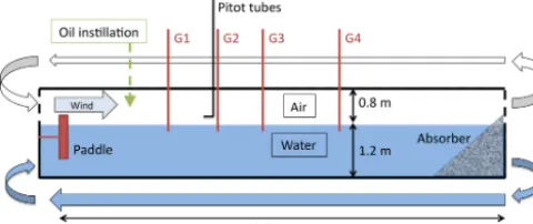
Figure 1. Schematic longitudinal diagram of the wave flume ar-rangement at the First Institute of Oceanography flume (Qingdao, P. R. China). For the sake of clarity, horizontal and vertical scales are distorted. The arrows indicate the direction of the flow.
pure frictional wind stress (which, in clean water, is not sep-arable from the wave stress), the related water surface drift, and the growth of irregular long waves under the action of the wind, by largely cancelling the short-wave roughness.
The paper is organized as follows. Section 2 gives a gen-eral description of the experimental set-up in the tank, lists the general plan of experiments with wind and paddle waves in clean water and with oil, and describes the water elevation and airflow data collected during the tests. The results of the experiments are examined in Sect. 3, where we show the re-sponse of the coupled air–water system to the presence of fish oil slick. The principal results and implications for air–water interaction studies of the present investigation are discussed in Sect. 4. Finally, the main findings of the study are summa-rized in Sect. 5. The paper is complemented by two videos recorded during the experiments showing the effect on wind and paddle waves of the surface layer of fish oil (Benetazzo et al., 2018b, c).
2 Experiment
2.1 The experimental set-up
The experiments described in this study were performed in a large wind- and paddle-wave facility allowing the gener-ation of winds at velocities comparable with those in open sea (but not extreme conditions). The measurements were carried out in the flume of the First Institute of Oceanogra-phy (FIO, Qingdao, P. R. China) illustrated schematically in Fig. 1. The tank dimensions are 32.5 m in length, 1.0 m wall-to-wall cross section, 0.8 m ceiling above the mean water sur-face. The water depth is 1.2 m, satisfying the deep-water con-dition for the wind-driven gravity–capillary waves, and prac-tically also paddle waves, analysed in this study. The smallest longitudinal natural frequency of the tank is 0.052 Hz. Side walls are made of clear glass to enable visualization of the wave field. A water pipe parallel to and below the flume al-lows continuity between the two ends of the tank.
The wind tunnel is mounted atop the wave tank, which is closed with side glass walls and a ceiling. The airflow could be driven up to a reference speed of 12 m s−1. Mechanically generated (paddle) waves coexisting with wind waves could be generated by a piston-type paddle in the range of periods from 0.5 to 5.0 s (frequencies from 0.2 to 2.0 Hz) and dissi-pated at the downwind end of the tank on a sloping beach of fibrous matter. Four calibrated capacitance-type wave gauges (featuring a linear response and accuracy of 0.3 mm) col-lected synchronous water surface elevation data for 300 s at 50 Hz at fetchesX=8.0 m (probe G1), 12.0 m (G2), 15.5 m (G3), and 20.5 m (G4) along the tank main axis. The fetch X=0.0 m corresponds to the inlet for wind in the water tank. For the statistically steady part of the wave records, the vari-ance frequency spectrum of water surface elevationz(t )was computed by means of the Welch (1967) overlapped segment averaging estimator (eight segments of equal length, 50 % overlap, Hamming window).
For characterization of the vertical profile of the along-channel component of the airflow velocity, five Pitot tubes sampling at 1/7 Hz were located atX=11.5 m in the cen-tre of the cross section and distributed at different heightsh above the still water surface, respectively (from tube 1 to 5) ath=8.3, 18.3, 28.3, 38.3, and 48.3 cm. Estimates of the wind stress were derived by fitting the Pitot tube observa-tions with a logarithmic law function ofh. For an aerody-namically rough airflow, the mean value of the along-channel component of the wind velocity U in the outer turbulent layer at heighth above the boundary is expected to follow a self-similar Kármán–Prandtl logarithmic law as a function of height
U (h)=u∗ κ log
h
h0
, (1)
where the overbar indicates the temporal averaging process, u∗ is the friction velocity along the same direction as U, κ=0.41 is the von Kármán’s constant. The non-zero param-eter h0 has the meaning of the roughness height where U appears to go to zero, namelyh0is the virtual origin of the mean velocity profile. In the presence of waves, the shape of the wind velocity profileU (h)is governed by both turbulent and wave-induced momentum flux, the latter being a func-tion of the wind input source term in Eq. (A2). The trans-port of horizontal momentum due to molecular viscosity is considered negligible, except very near the surface where the vertical motion is suppressed. The total air-side shear stress τaat the boundary of the flow is then approximated as
τa=ρau2∗ (2)
withρabeing the air density.
wa-ter surface drift velocityuw0constitutes the boundary condi-tion at h=0 for the vertical profile of the airflow velocity. Wu (1975) found that at the air–water interface, the wind-induced current is proportional to the friction velocity of the wind, and it is associated with the wind shear, Stokes drift, and momentum injection during wave breaking events. For non-breaking wavy surfaces, the wind-induced surface cur-rent was determined to be around 50 % of the airflow friction velocity (Phillips and Banner, 1974; Wu, 1975). In a clean-water wind-wave tank and at steady conditions, the value of uw0can be related to the maximum value ofUa(h). This is not achieved at the largest distances from the water due to the presence of the tank roof. Auw0value around 3.3 % of the free-stream maximum wind velocity seems to be a reason-able approximation (Liberzon and Shemer, 2011; Peirson, 1997; Wu, 1975) and was used in this study. The accuracy of the wind stress obtained from the profiles measured by Pitot tubes in a wave tank was examined by Liberzon and She-mer (2011), who found that the values of the wind stress ob-tained from the measurements by the Pitot tube and those cal-culated from the Reynolds stresses agree within about 10 % mean difference (using an X-hot-film thermo-anemometer).
A series of videos showing the water surface conditions in clean water and in water with oil complements the available data providing a plain perception of the fish oil effect on the surface waves.
2.2 The experiments
Our experiments aimed at analysing the different results, us-ing the different combinations of reference wind speed Ur, paddle waves (changing the peak wave periodTpand the sig-nificant wave heightHs), and oily surface. The data of each experiment were later screened for correct data availability and consistency among the different instruments. This led us to exclude several records considered not suitable (indepen-dently of the physical results) for the final analysis. This was based on the six experiments listed in Table 1. Two differ-ent blower reference speeds were analysed, namely Ur=6 and 8 m s−1, and one set of irregular paddle waves (JON-SWAP spectrum withTp=1.0 s andHs=6.2 cm; steepness Hs/Lp=0.04 with Lp being the peak wavelength). Note that many of these experiments have been repeated up to four times. All experiments were initiated with no wind and undisturbed water surface.
Three experiments were made with the fish-oil-covered water surface (two with wind waves and one with wind and paddle waves). The dilational modulus ε of this type of oil is roughly 0.03 N m−1 (Foda and Cox, 1980); hence its resonance frequency given in Eq. (A1) is estimated to be ωres=23.7 rad s−1, i.e. linear frequency of 3.77 Hz and wavelength of about 11 cm. Moreover, the radial spreading speed of fish oil is around 0.14 m s−1, sufficiently large to keep uniform the oil film that might be broken by the wave action (Cox et al., 2017). Before performing the experiments
with the slick-covered surface, the oil was instilled from the ceiling at a fetchX=4 m, releasing 26 drops with the blower at rest. Estimating each drop of volume about 50×10−9m3, the average oil thickness on the water surface was 4×10⁻⁸m, namely a few molecular layers. During experiments W06-O and W08-P-O, the oil film was preserved by continuously in-stilling surface oil drops onto the water, while the dropping was interrupted (no instillation) at the onset of the wind start in the experiment W06-O-NI (see Table 1).
A crucial point in wind-wave tank measurements concerns the correct reference system for waves generated by wind. The wave data acquired by the probes in the tank are repsented in a fixed (absolute) reference system, while the re-sponse of the wave field to the oil film is intrinsic to the wave dynamics. Therefore the sea surface elevation energy spec-trumEmust be mapped in a reference system moving with the wind-generated near-surface water current. To this end, the wave spectrum must therefore be transformed from abso-lutefato intrinsic frequenciesfi, i.e. those that would have been recorded by a probe moving with the current. Indeed, for waves propagating over a moving medium, the Doppler effect modifies the observed frequency of each elementary periodic wave that makes up the random wind field (Lind-gren et al., 1999). This effect can be particularly large for short waves at sea (hence modifying the slope of the high-frequency spectrum tail; Benetazzo et al., 2018a), and also in a wave tank where waves are generally short whilst the cur-rent speed can be a non-negligible fraction of the wave phase speed.
For harmonic waves at the limit of small-wave steepness and neglecting the modulation of short waves by long waves (Longuet-Higgins and Stewart, 1960), the relation between faandfiis given by (Stewart and Joy, 1974)
fa−fi−[kuwcos(θ−θU)]/(2π )=0, (3)
whereuwis an appropriate water velocity vector of direction θU, andθthe wave direction (Kirby and Chen, 1989; Stewart
and Joy, 1974). At the leading order, it is assumed that the dispersion relationship of the gravity–capillary-wave theory provides a unique relationship between the frequencyfiand the wavenumberkas follows:
2π fi=
s
gk+T ρk
3 (4)
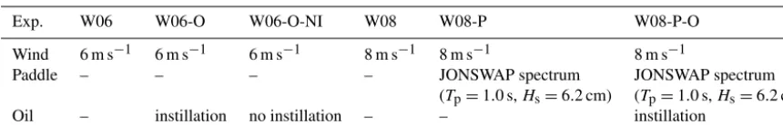
Table 1.List of experiments performed in the wind- and paddle-wave tank, using clean water (ordinary tap water) and after instilling fish oil. The wind speed is the reference valueUrimposed at the blower. For paddle waves,Tpis the peak period andHsthe significant wave height. Blanks denote not applicable cases.
Exp. W06 W06-O W06-O-NI W08 W08-P W08-P-O
Wind 6 m s−1 6 m s−1 6 m s−1 8 m s−1 8 m s−1 8 m s−1
Paddle – – – – JONSWAP spectrum JONSWAP spectrum (Tp=1.0 s,Hs=6.2 cm) (Tp=1.0 s,Hs=6.2 cm) Oil – instillation no instillation – – instillation
intrinsic coordinates can be derived as
E(fi)=E(fa)Jai, (5)
whereJai= |dfa/dfi|is the Jacobian of the transformation, which in the limit of deep water can be written explicitly as
Jai=
1+2uw
s
gk+T ρk
3/
g+3T ρk
2
. (6)
3 Results
3.1 Wind waves without and with oil
We begin the examination of the change of gravity–capillary-wave properties caused by the fish oil film by analysing the effects on the water elevationzand wind speed profileUa(h) during experiments W06 (Ur=6 m s−1and clean water) and W06-O (the same as W06 but with oil slick). For the lat-ter, the wind-wave field attenuation due to the Marangoni forces is readily visible in Fig. 2, which shows two pictures of the water surface without (Fig. 2a) and with (Fig. 2b) oil instillation. After the oil film is spread on the water, the surface is largely smooth with only tiny elevation os-cillations (1 mm at most; see Fig. 4) and there appears to be no organized wave motion (see also the video supple-ment: https://doi.org/10.5281/zenodo.1434262; Benetazzo et al., 2018b). It is obvious that the presence of an extremely thin, practically monomolecular, layer of oil on the surface greatly alters the air–sea interface properties. We analyse the situation first from the point of view of the air, and then from the water.
3.1.1 Airflow characterization
We begin evaluating the air-side stress due to the wind drag on the water surface. In the W06 experiment the maximum Ua(h) value of 6.06 m s−1 was found, attained at the third Pitot tube, namely at h=28.3 cm from the still water sur-face. Hence, accounting for a surface water speed uw0= 6.06×0.033≈0.2 m s−1, a logarithmic curve was fitted (the mean absolute error of the fitting is 0.01 m s−1) to the average profile U (h)=Ua(h)−uw0 and the two parameters u∗=
0.29 m s−1andh0=0.1 mm were estimated accordingly. For
the lowest Pitot tube (h=8.3 cm), the dimensionless height h∗=gh/u2∗ is 9.7, implying that from there upward wind
data were collected in a region where turbulent stresses are expected to dominate over wave-induced stresses (Janssen and Bidlot, 2018). The typical viscous sublayer thickness approximated as 11.6ν/u∗measured 0.6 mm, and the
atmo-spheric boundary layer may be characterized as aerodynam-ically smooth. The wind shear stressτa based on the mea-surement in this layer equals 0.10 N m−2. The equivalent wind speed at heighth=10 m, extrapolated from Eq. (1), is U10=8.6 m s−1, which is in satisfactory agreement with the typical relation betweenu∗ andU10 found in a wind-wave tank filled with clean water (Liberzon and Shemer, 2011; Mitsuyasu and Honda, 1986). The neutral drag coefficient measured at 10 m height and defined asCD= u∗/U10
2 is 1.1×10⁻³. The values ofu∗ andh0are in agreement with those obtained in the experimental results by Liberzon and Shemer (2011), and those estimated by the bulk parameter-ization of air–sea turbulent fluxes provided by the Coupled Ocean–Atmosphere Response Experiment (COARE) algo-rithm (Fairall et al., 2003) that givesτa=0.11 N m−2, using as input theU (h)profile determined in our experiments.
The smoothing of the water surface in the presence of oil reflects on the airflow, which differs from that over clean wa-ter and has a smaller vertical gradient dUa/dhof the wind speed (Fig. 3). Because of the reduction in the resistance on the water surface, the wind speed strengthens over the film-covered surface, but the effect is limited to the low-est part of the turbulent airflow. Similar behaviour was ob-served in the wind-wave tank experiments by Mitsuyasu and Honda (1986). For continuity reasons, i.e. for the practically constant airflow discharge in the tank (the difference of the discharges measured by the Pitot tubes is smaller than 1 %), a less steep wind profile implies a lower velocity with respect to the clean-water case in the central line of the flow (with oil the maximum value ofUa(h)was 5.91 m s−1).
Figure 2.Two photographs showing the water surface condition at a fetch of about 20 m taken without(a)and with oil instillation(b). In both cases the water surface was forced with a reference wind speedUr=6 m s−1(blowing from left to right in the pictures). The wave probe G4 is visible on the left-hand side of both pictures. The red arrow in the right panel points to the oscillating flow (vortex shedding) past the probe. See also the video supplement (Benetazzo et al., 2018b).
Figure 3.Vertical profile of the wind velocity componentUa mea-sured over the water surface at a fetchX=11.5 m. Reference wind speedUr=6 m s−1. Clean-water conditions (blue) and oil-covered surface (red). In the legend, the value of the airflow friction velocity u∗is shown within brackets. Only the values recorded at the three
lowest Pitot tubes are shown.
by wave breaking. In terms of spectral quantities the stress to the water columnτwcan be computed as
τw=τa−ρwg 2π
Z
0
kmax
Z
0 k
ω(Sin+Snl+Sdi)dkdθ, (7)
where we have omitted the direction of the flux that we as-sume aligned with the flume main axis. On the right side of Eq. (7), theS terms represent the net effect of sources and sinks for the wave energy spectrum (see Appendix A). In the high-frequency equilibrium range, the momentum com-ing from the wind and non-linear interactions is dissipated and is therefore directly transferred to the water column.
The balance in Eq. (7) is plainly altered for an oil-covered surface, as it is visible in Fig. 2b, for which we assume Sin+Snl+Sdi=0. In this case, the wave-induced transport is practically null, and the total current drift is supported only by the stressτaexerted by wind at the air–sea interface. In this respect, from visual inspection of the supporting videos acquired during the experiments, we did observe the pres-ence of a water surface drift and a high-frequency oscillating flow downstream from the probes’ beams (the vortex shed-ding at G4 is pointed out by the red arrow in Fig. 2b; see also the video supplement; Benetazzo et al., 2018b). The lat-ter implies the presence of a near-surface drift impacting the probes. No adequate instrumentation (e.g. particle image ve-locimetry; e.g. see Adrian, 1991) had been designed in ad-vance to obtain a representation of the fluid flow close to the wavy air–water interface.
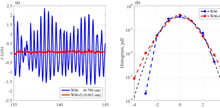
(di-Figure 4.Sea surface elevation for clean (blue) and slick-covered (red) surface.(a)Excerpt of the single-point recordz(t )atX=20.5 m (probe G4) for the two conditions with clean water (experiment W06) and after the oil instillation (W06-O). In the legend, the value of the standard deviationσofz(t )is shown within brackets.(b)Histogram of the normalized elevations, high-pass filtered above 1 Hz. The black dashed line shows the Gaussian probability density function (pdf).
ameter d=4 mm). Use of the related vortex shedding fre-quencyf ≈0.21uw0,oil/d (see later in Sect. 3.1.2) suggests uw0,oil=20 cm s−1, which is close to (actually less than) the estimate using bubbles, which probably were also partially drifted by wind.
With this information, we have found that the wind stress for an oil-covered smooth surface is τa,oil=0.005 N m−2, approximately 5 % ofτa, and the drag coefficient undergoes a decrease of 1 order of magnitude. The extrapolated 10 m height wind speedU10,oilis 6.3 m s−1, smaller thanU10, in contrast to the field observations of Ermakov et al. (1986), most likely because our observations were collected in a tank with an upper roof. The roughness height was determined to beh0<10−6m, implying that the air boundary layer for the oil-covered water shows properties of a hydrodynami-cally smooth flow. This result complements those of Mit-suyasu and Honda (1986) and MitMit-suyasu (2015), who ob-served that for low wind speeds (few metres per second) and short fetches the water surface aerodynamic properties are similar in clean water and in water with surfactant. Indeed, in those studies the surfactant only partially suppressed the wind-wave field, while, on the contrary, the use of fish oil in our experiments cancels the wind-wave generation process such that the water surface is felt as smooth by the airflow.
3.1.2 Wave field characterization
In the presence of the viscoelastic oily film, the gravity– capillary-wave damping is quantified by analysing the time records z(t ) of the sea surface elevation field at different fetches. In this respect, Fig. 4a gives a clear idea of the Marangoni damping effect, which can be quantified by
not-ing that the standard deviation σ of z(t ) shrinks by 1 or-der of magnitude. However, the process involves more than a decrease in the vertical oscillations, as it is the whole spatio-temporal distribution of the surface elevations that is abruptly changed (Fig. 4b). Indeed, whereas in clean water, in active wave generation, the histogram ofz(high-pass fil-tered above 1 Hz; see discussion below) has a positive skew-ness coefficient, as is expected for wind waves (Longuet-Higgins, 1963), in the presence of oil the empirical histogram is quasi-symmetric around the mean (the skewness coeffi-cient is−0.03, very close to zero). This implies that for slick-covered surfaces the generation and evolution of gravity– capillary waves are governed by a different balance and pro-cess, which are dominated by the reduced wind input and the Marangoni energy sink, which lead to a quasi-Gaussian sur-face elevation field at all scales.
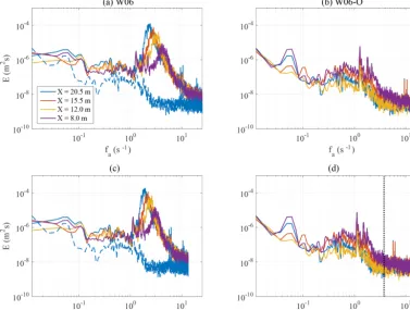
over-Figure 5.Wave energy spectraE(fa)andE(fi)of the water surface elevationz(t )at different fetches. Reference wind speedUr=6 m s−1. (a, c)Clean-water experiment W06.(b, d)Water with oil experiment W06-O (the spectrum at the fetchX=20.5 m is replicated with a dashed blue line in panelsaandc). The vertical grey dotted line in panel(d)shows the fish oil resonance frequencyfres=ωres/(2π )=3.77 Hz.
shoot of the peak of the spectrum. The total wave energy increases with fetch: the significant wave height Hs grows from 1.21 cm at the shortest fetch (X=8 m) to 3.16 cm at X=20.5 m. It is remarkable that for the slick-covered sur-face, there is no evidence of wave growth with fetch (Fig. 5b and d).
Focusing for the time being on the comparison among the oil and no-oil cases, the differences are obviously macro-scopic, but it is worthwhile to analyse them for different fre-quency ranges. For low frequencies, say below 1 Hz, there is clearly some energy also in the oil spectra. Note the peaks around 0.05 Hz in the G1 and G4 spectra, reduced in G2 and G3. Remembering (see Sect. 2) the longitudinal natu-ral frequency of the tank, we interpret these as “seiches” of the wave tank, obviously more visible the further the gauges are from the centre of the tank. In the clean-water case more distributed oscillations exist, which we associate with a more active action of a possibly irregular wind flow. The most in-teresting range is of course between 1 and 4 Hz (close to the fish oil resonance frequency). Here the effect of oil is macroscopic, with oil-case energy several orders of magni-tude smaller than without oil. Finally, still for the oil spectra, no wave signal is visible above 3–4 Hz where we expect the maximum damping of surface waves due to the oily surfac-tants (Alpers and Hühnerfuss, 1989).
A more direct comparison between the W06 and W06-O spectra is shown in Fig. 6 for each frequency, showing the ratio of the respective spectral energies. If we represent the frequency- and fetch-dependent damping coefficient as the ratioD(fi, X)=Eo/Ecbetween the variance density spec-trum of the water surface elevation with oil slick (Eo) and in clean water (Ec), we then findDvalues as small as 10−4at the longer fetches. Of course the maximum differences are at the peak frequency of the no-oil spectra, the respective frequency and ratio decreasing with fetch while the no-oil energy increases.
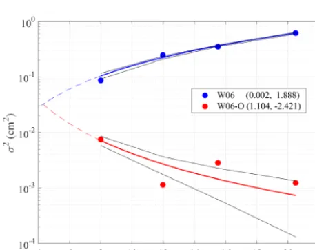
To interpret the data from the experiments we analyse how wave energy depends on fetch. In Fig. 7 we show how the corresponding surface elevation (high-pass filtered above 1 Hz) variance σ2= h(z(t )− hz(t )i)2i (the angle brackets, hi, denote the ensemble average) varies for the clean water and oil cases. Assuming the different orders of magnitude, it is macroscopically observed that while the wave energy in clean water grows with fetch, the opposite is true (or is suggested to be) with oil. To better quantify the fetch depen-dence, we have fitted a power law,
Figure 6.Damping of the wave energy for oil-covered water sur-face. The damping coefficient is evaluated as the ratioD=Eo/Ec between the variance density spectrum of the water surface eleva-tion with oil slick (Eo) and in clean water (Ec). The thin solid black line shows the levelEo=Ec.
Figure 7.Spatial evolution of the water surface elevation variance σ2 (filled symbols) in clean water (W06) and with fish oil slick (W06-O). The solid blue and red lines are the power-law-type func-tionσ2=αXβ fitting the observations (in the legend, the coeffi-cientsαandβare tabulated), while the dashed lines show the laws extended outside the observed data interval. The root-mean-square error for the fitted function is 0.027 and 0.002 cm2 for W06 and W06-O, respectively. The black lines show the prediction bounds (confidence level of 50 %) for the fitted curves.
to the water surface varianceσ2versus fetchX. The best fit parametersαandβare tabulated in the legend of Fig. 7 (with σ2in square centimetres andXin metres).
Extrapolated backwards out of the experimental range in the figure, the two fitted laws intersect each other around X=4 m. This is the fetch at which oil was introduced into
the tank. Note that in the W06-O experiment oil was con-tinuously instilled during the experiment. This was because the wind, acting on the surface oil and creating (as we have seen) a current, tends to push it along the tank faster than the oil tends to distribute uniformly on the surface (with radial speed around 14 cm s−1). Indeed this is smaller than the sur-face speed derived in the previous subsection for the oil case. While the continuous, although very limited, instillation of oil during W06-O ensured the presence of an oil film from the instillation point onwards, the wind, acting from fetch X=0 m, was pushing the oil away from the first 4 m zone where waves could be generated; hence equal in both the oil and the no-oil cases. Therefore the oil-case energy we see in Fig. 7 at 8 m fetch is the remnant of the one previously generated and already partially dissipated between the 4 and 8 m fetches due to the acting Marangoni forces. This explains why the highest energy in the oil spectra is in the first spec-trum, i.e. the shortest fetch.
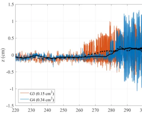
The shift along the tank of the surface oil film due to the wind drag is also well illustrated by the results of the W06-O-NI experiment, i.e. when, starting with a layer of oil well distributed on the water surface in the tank, we did not further instill oil during the action of the wind (reference wind speed Ur=6 m s−1). The resulting records atX=15.5 m (G3) and 20.5 m (G4) are shown in Fig. 8. It is obvious that around 262 s the effect of oil is beginning to vanish at G3, followed 15–20 s later by a similar result at G4. Note that this does not mean the whole oil was pushed past G3 at 262 s. Were this the case we should see in the record the already gener-ated waves (up to position G3). Rather, the oil edge is getting close enough to let G3 feel the consequences, which are dif-ferent from those at G4: in the range [290, 300] secondsHs grows from 1.56 cm (G3) to 2.34 cm (G4), conveying the fact that a longer fetch was progressively made clean by the near-surface water drift. The progressively increasing space free of oil is also manifest in the record of each probe, where the basic wave period tends to increase with time.
In the W06 experiment, spectra at the longer fetches show two highly energetic and very close peaks around the fre-quencyfa≈10 Hz (probes G3 and G4, see Fig. 5). As men-tioned in Sect. 3.1.1, our interpretation is that they are orig-inated by the vortex-induced vibrations at the cylindrical holding beams of the probes. Indeed, the frequency fv at which vortex shedding takes place is related to the Strouhal number by the following equation:
St=fvd
u , (9)
ev-Figure 8.Sea surface elevation at probes G3 (X=15.5 m) and G4 (X=20.5 m) for an initially slick-covered surface without oil in-stillation (experiment W06-O-NI). The dashed and solid black lines show the smoothed elevations (moving average of size 5 s) at G3 and G4, respectively. In the legend, the variance inz(t )within the range of 290 s≤t≤300 s is reported.
idence. Elaborating this point further, it is worth noting that similar spectral peaks (as energy and frequency) have been also found during the W06-O experiment. In our interpre-tation, this evidence supports the fact that the water surface drift was generated by the wind friction also in the presence of oil, and that its magnitude is consistent with one expected in clean-water conditions.
3.2 Wind and paddle waves without and with oil The second series of experiments was done by adding me-chanically generated paddle waves to the wind-generated ones, both in clean water and in water with fish oil. We had two specific purposes. The first one was to explore the influ-ence of pre-existing relatively long waves (the paddle gener-ated ones) on the local generation of wind waves. The sec-ond purpose was how this interference was modified by the presence of fish oil. This second set of experiments (namely W08-P and W08-P-O) was done with an 8 m s−1reference wind speed. A 6 m s−1reference speed would have allowed a more direct comparison with the results obtained without paddle waves (previous section). At the same time, a higher wind speed was useful to better highlight the interaction with the paddle waves.
In the tank, paddle waves were generated as a JONSWAP spectrum with nominal 6.2 cm significant wave height and 1.0 s peak period. On top of this, wind waves were gener-ated by the wind. The resulting surface wave field is shown in Fig. 9a, the picture being taken, as Fig. 2, close to fetch X=20.5 m. Starting with a qualitative perception from the image (see also the video supplement; Benetazzo et al.,
2018c), we derive, as expected from what is reported in the literature, that wind waves grow substantially less than ex-pected in a pure wind sea (Wu, 1977). For a full compar-ison we also ran the W08 experiment, with wind blowing at Ur=8 m s−1 without paddle waves and in clean water. The comparison between Figs. 2 and 9 is even more strik-ing considerstrik-ing the larger wind speed in Fig. 9. Clearly, the presence of the paddle waves has an effect. This is a matter of practical relevance for the cases when in the ocean fresh new waves are generated and superimposed on a pre-existing swell (in this case propagating along the same direction). A more quantified comparison of W08-P and W08 (i.e. with and without paddle, respectively) is provided by the wave spectra shown in Fig. 10. We see that the introduction of the irregular paddle waves cancels the wind wave peak of W08 at about 1.6 Hz. However, the tails of the two spectra some-how converge above 2.2 Hz. As we will soon see, with paddle waves the conditions did not allow the visual measurement of current.
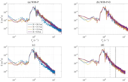
We analyse how the overall effect varies with fetch (both without and with oil). The related spectra are depicted in Fig. 11. Contrarily to the pure windy cases (experiments W06 and W08), there appears to be no evident dependence on fetch of the wave energy. Our interpretation is the fol-lowing. On the one hand, the disappearance of the wind sea energy peak in the presence of long waves implies that the wind wave peak does not develop with fetch. On the other hand, in water with oil, at higher frequencies the balance is between non-linear interactions and Marangoni dissipa-tion, which is only slightly depending on fetch. Note that, as clearly represented in Fig. 12, the attenuation is maxi-mum around 3 Hz (smaller than the resonance frequency) and the maximum damping (D) of wind wave energy (see for comparison Fig. 6) is 2 or 3 orders of magnitude smaller than with only wind waves (experiments W06). This is the consequence of two parallel facts: less wind wave energy in the presence of paddle waves and a decreased efficiency of damping by oil film, as is evident when comparing Figs. 2b and 9b. These effects also have an impact on the short wind waves, as the damping effect appears to cease at frequencies higher than 9 Hz (Fig. 12)
Figure 9. Two photographs of the water surface condition at a fetch of about 20 m taken without (a, experiment W08-P) and with oil instillation (b, experiment W08-P-O) onto wind waves (wind blowing from left to right of the pictures at the reference wind speedUr= 8 m s−1) and irregular paddle waves. See also the video supplement (Benetazzo et al., 2018c).
Figure 10.Variance density spectrumE(fi)of the water surface el-evationz(t )at a fetchX=20.5 m (wave probe G4) in the presence of coexisting wind and paddle waves in clean water (W08-P), wind and paddle waves in water with oil (W08-P-O), and wind waves only in clean water (W08). The dashed grey vertical line shows the maximum frequency (2 Hz) produced by the paddle.
the waves progressively decreasing with fetch (the coefficient β <0), consistently with, and with the same explanation for, the results obtained without paddle waves.
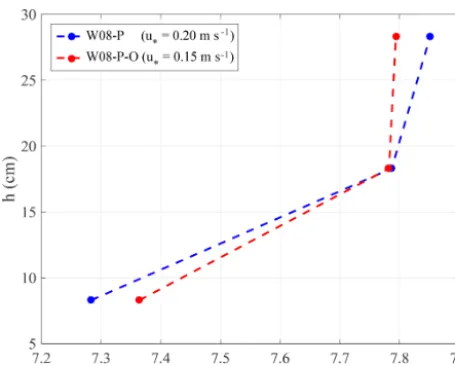
The growth of paddle waves under the wind forcing ap-pears to be marginally affected by the presence of oil (PW symbols in Fig. 13), generalizing to a more realistic wave field the results by Mitsuyasu and Honda (1986) obtained for monochromatic paddle waves. We interpret this by arguing that the reduction in surface roughness between W08-P and W08-P-O is not sufficient to substantially change the vertical profile of the turbulent airflow; hence the generation process acting on long waves. This is confirmed by Fig. 14 showing the wind profile with and without oil. There is only a small difference between the two cases; however, the friction ve-locity is, as expected, larger in clean water. This implies that
the minor disturbances we see in the Fig. 9b suffice for mak-ing the wind feel the surface as rough. Indeed we are at the limit because the further, almost complete, wave reduction we see in Fig. 2 for the experiment W06-O changes dramati-cally the wind profile, as already seen in Fig. 3.
4 Discussion
Our previous description of the general methodology and re-sults were focused on the implications of having the water surface covered by a very thin (∼10−8m) layer of fish oil. However, interesting in itself, it is clear that the main virtue of these experiments has been the opening of new perspec-tives on the physics of air–sea interactions. We discuss here the main suggestions and ideas derived from our results.
– The different wind profile and wave growth without and with oil clearly show that the stress felt by the atmo-sphere is, as anticipated by Janssen (1991), the sum of the friction stress and the input to waves. Lacking the latter, the atmospheric stress reduces to the purely frictional one. This also has implications for circulation modelling where quite often the wave intermediate role (wind input to waves followed by wave input to cur-rent via breaking) is bypassed by an artificially inflated surface friction to current. In this respect, McWilliams and Restrepo (1999) showed how the general global cir-culation could be obtained by also driving it only with breaking wave momentum injection.
Figure 11.Wave energy spectraE(fa)andE(fi)of the water surface elevationz(t )at different fetches for the reference wind speed of 8 m s−1and irregular paddle waves.(a, c)Clean-water experiment W08-P.(b, d)Water with oil experiment W08-P-O (the spectrum at the fetchX=20.5 m is replicated with a dashed blue line on the left panel). On bottom panels the dashed grey vertical line shows the maximum frequency (2 Hz) produced by the paddle, and the dotted black vertical line on the bottom-right panel shows the fish oil resonance frequency fres=ωres/(2π )=3.77 Hz.
Figure 12. Damping of the wave energy for an oil-covered wa-ter surface. The damping coefficient is evaluated as the ratioD= Eo/Ecbetween the variance density spectrum of the water surface elevation with oil slick (Eo; experiment W08-P-O) and in clean wa-ter (Ec; experiment W08-P). The thick solid black line is the aver-age shape of the damping coefficient (for the sake of clarity the se-ries is smoothed with a moving average procedure). The thin solid black line shows the levelEo=Ec.
Figure 14.Vertical profile of the wind velocity componentUa mea-sured over the water surface at a fetchX=11.5 m for coexisting wind- and paddle-generated waves in clean-water condition (blue) and for oil-covered surface (red). In the legend, the value of the fric-tion velocity is shown within brackets. Only the values recorded at the three lowest Pitot tubes are shown.
the current vertical profile, and supported also by the re-circulation characteristics of the wave tank, we made the blunt assumption of a vertically uniform current. This is a first-order approximation that we consider acceptable in our case because the related discussion concerns only very short waves. In any case, more complete experi-ments are planned for the near future.
– We have found it interesting to look at how the water surface reacts and evolves under the action of an im-pulsive wind forcing. For this first analysis of the ob-tained data, we have limited ourselves to the steady, fetch-limited conditions. This subject takes us to a very short discussion on the generation mechanism(s) of the earliest waves. In this respect, the spectral approach to wind wave modelling began with the study by Pierson et al. (1955), followed by the two parallel and indepen-dent, but complementary, papers by Phillips (1957) and Miles (1957), and the definition of the energy balance equation by Gelci et al. (1957). While the Miles mecha-nism, refined by Janssen (1991), provides the bulk of the input to waves, we still need to trigger the first wavelets on which the mechanism, and non-linear in-teractions, can then act. Two processes compete for this first stage: the just mentioned one by Phillips, associ-ated with assumed pressure oscillations moving with the wind, supported also by the recent paper by Zavadsky and Shemer (2017), and a sort of Kelvin–Helmholtz in-stability (Kawai, 1979) due to the strong vertical shear in the surface water layer following the initial action by wind. The matter is not relevant for practical
pur-poses because these initial stages are usually parame-terized or bypassed in wave modelling in a pragmatic way. We know these wavelets appear and their exact di-mensions are irrelevant for the following evolution of the actual field. In this regard, our experiments provide a small piece of information. The Phillips mechanism is supposed to act on any wavelength, independently of the other ones. We argue that in the oil experiment, as-suming the dissipation at the wavelet scale due to the Marangoni effect, nothing would impede the Phillips mechanism to act on the longer waves. However, we found no evidence of energy in the corresponding wave components.
– With short wind waves and long paddle waves, the pres-ence of oil still reduces wind-wave generation, but there is more wind-wave energy than with only wind. There-fore the presence of a swell reduces the effectiveness of the oil impeding local generation. We hypothesize that this is mainly due to the long wave orbital motion that detunes the resonance conditions between Marangoni waves and gravity–capillary waves. Moreover, this mo-tion continuously disrupts the continuity of the oil layer and hence the effectiveness of the Marangoni forces.
5 Conclusions and summary
With the help of an experimental facility, we have studied the influence of a very thin layer of fish oil on wind and paddle waves as well as on the parameters of the lowest air-flow layer. Measurements of sea surface elevation at different fetches and wind speeds were carried out in both clean wa-ter and in wawa-ter with fish oil producing a viscoelastic film on the surface. The damping of short gravity–capillary waves by surfactants appears to be a convenient condition to study, to a large extent, the processes of interaction between the water body and the atmosphere. The aim of the present study is thus to evaluate the influence of the fish oil film on the growth of wind and paddle waves and on the air–water interaction pro-cess. Taking this viewpoint, the principal conclusions of our study can be summarized as follows:
– Our results show the efficacy of fish oil in suppressing wave generation by wind. Indeed, in the experiments in a wind-wave tank contaminated by non-animal sur-factants, Hühnerfuss et al. (1981) found that the peaks of the spectra are shifted towards higher frequency when compared with clean-water conditions. However, a wind-wave spectrum was still present in their tests, whilst we have found that, using fish oil in the wind-only condition (reference wind speed of 6 m s−1), the wave field does not grow from the rest condition, lead-ing to a strong modification of the airflow vertical pro-file.
– The experiment with wind-wave only in water with fish oil (experiment W06-O) gave us the unique opportu-nity to investigate (albeit preliminarily) the interactions at the air–water interface in absence of surface waves. Clearly, the stress exerted in that case by the airflow is smaller than the stress in clean water (when the wave field regularly develops) and the water current is de-termined by the wind shear only so that τw≈τa. This condition is expected to be different from the condi-tion obtained for fully developed waves (in clean wa-ter), when one should find that in Eq. (7) the momen-tum flux into the water column τw should become the atmospheric stressτaas the wave field reaches equilib-rium (see ECMWF, 2017). For instance, the water cur-rent vertical profile below the surface is expected to be different in clean water and in water with oil. In this respect, new experiments are already planned that will also investigate the drift current distribution beneath the water surface for an oil-covered water surface.
– The growth of long paddle-generated waves seems to be less affected by the roughness of short waves. Provided a minimal background of very short waves (in prac-tice surface roughness) is present, the growth of paddle waves under the action of wind is largely independent of the background roughness, a fact we ascribe to the similar distortion of the wind profile in the two cases. With our study we have shown that wave generation and dis-sipation, and more general atmosphere and sea dynamic in-teraction, are still to be fully explored. The approach we fol-lowed, experiments in a wind-wave tank without and with oil on the surface, offers new possibilities for studying this old, but still fruitful, field.
Appendix A: The Marangoni wave damping effect The physics of the Marangoni effect is well understood, and it is generally agreed that the gravity–capillary-wave energy is damped by a surfactant by the following mechanism. Im-mediately after a wave field enters a surfactant patch, the Marangoni effect due to the viscoelastic film on the water surface increases viscous dissipation of short wave energy at specific frequencies. This is caused by an additional dissipa-tion in the surface boundary layer. Indeed a shear stress in the boundary layer is required to balance the stress due to the surface tension gradients originated by the non-uniform concentration of the surface viscoelastic film (alternatively contracted and expanded due to the passage of a wave). This gives rise to additional longitudinal waves in the boundary layer superimposed on the existing surface waves that are thus damped by a resonance-type mechanism. The dissipa-tive spectral sink (the so-called Marangoni resonance re-gion) is at frequencies between 3 and 8 Hz, the scale of the maximum damping depending on the dilatational mod-ulus of the surfactant (Alpers and Hühnerfuss, 1989; Fis-cella et al., 1985). The resonant angular frequency ωres for the Marangoni-force wave damping is given by
ωres=
(
cos(π/8)4g4(ηρw) ε2
)15
(rad s−1), (A1)
whereg(m s−2) is the gravity acceleration,ρw(kg m−3) the clean-water density,η(Ns m−2) the clean-water dynamic vis-cosity, andε(N m−1) denotes the dilatational modulus of the surface film. As stated by Eq. (A1), the larger the modulus εthe longer the damped waves. The maximum damping of gravity–capillary waves is attained at a frequency lower than ωres(the Marangoni wave is a strongly damped wave) and the width of the resonant damping is quite broad (the half-power width is of the order of 1 to 2 Hz; Alpers and Hühnerfuss, 1989).
In a more formal approach, the description of water sur-face gravity waves generally follows a statistical approach by means of the development of the wave elevation variance spectrumE=E(k, θ;x, t )in the physical spacexand time t (kis the wavenumber andθthe propagation direction), its evolution governed by the energy balance equation (Gelci et al., 1957). In deep waters, it reads
∂N ∂t +
∂N
∂x ·(xN )˙ =Sin+Snl+Sdi, (A2) where N=E/ω is the wave action density spectrum with ω the intrinsic angular frequency. Furthermore,x˙=cg+U withcgthe wave group velocity andU an appropriate cur-rent. The right-hand side of Eq. (A2) represents the net ef-fect of sources and sinks for the spectrum (Komen et al., 1994): Sin is the rate of energy transferred from the wind to the wave field,Snl is the rate of non-linear energy trans-fer among wave components with diftrans-ferent wavenumber, and
Sdi=Sdi,b+Sdi,v is the rate of energy dissipation due to breaking (Sdi,b) and viscous forces (Sdi,v).
In our experiments the observations dealt with in this paper are the ones collected at steady state so that the spectrum at any fetch is determined by the upwind evolution of the source functionsSin,SnlandSdi; that is,
N= x
Z
0
h
cg+U
−1
(Sin+Snl+Sdi)
i
dx, (A3)
where, with good approximation, we have neglected the cross-tank wave energy evolution. The velocitiescg andU are also, but very weakly, fetch dependent. The balance in Eq. (A3) indicates that any modification of the wave energy may and must be caused by changes in the rate of wind input, dissipation, and/or non-linear transfer.
In the presence of oil, all three source functions undergo a change compared to the clean-water condition. Indeed, the rapid suppression of short waves by Marangoni forces re-duces the water surface mean slope, which leads to a change in the wind vertical profile and rapid decrease in the momen-tum flux from the wind to the wave field (e.g. see Mitsuyasu and Honda, 1986). Those two effects combined produce a change in the shape of the wave spectrum in the equilibrium range, which leads, via non-linear wave–wave interaction (Hasselmann, 1962), to a slow leakage (but fast compared to the pure viscous one; Alpers and Hühnerfuss, 1989) at wave-lengths longer than those at which the Marangoni forces are effective.
Given the possible variability in the surfactant density on the water surface, it is natural to wonder about the related sensitivity of the effect on waves. Analysing the wind-wave tank experiments with surfactants (sodium lauryl sulfate) presented by Mitsuyasu and Honda (1986), we can distin-guish two different regimes for wave attenuation, which cor-respond to weak and strong wave damping. Firstly, for small surfactant concentrations (i.e. weak damping), the peak fre-quency of the wind-wave spectrum in the presence of films is shifted to higher frequencies relative to the peak frequency of clean water (in other words waves develop more slowly). However, spectra preserveu∗similarity, and the new spectral
shape was ascribed mainly to the decrease in the wind stress: the surfactants smooth the surface and act to reduce the wind stress; therefore, the waves grow less. We interpret this result assuming that for low surfactant concentrations the effective-ness of the Marangoni damping is small (i.e. the water sur-face is not fully covered by a uniform film), but with a par-tially reduced aerodynamic roughness. On the contrary, for the highest concentration (hence with a strong damping) the similarity no longer holds, and most of the energy around the peak is lost (the maximum energy is at a frequency smaller than the one in clean water; see also Figs. 5 and 6).
Appendix B: Surface current drift estimate using optical flow
As it is specified in Sect. 3.1.1, tiny bubbles moving on the surface along the tank, and visible in the 1920×1080 pixel images captured at 60 Hz by a video camera placed outside the tank close to prove G4, made it possible to have an es-timate of the water surface current. The probe’s two vertical wires, whose dimensions have been accurately determined, were used to map visual features from the image space (in pixels) to the tank surface space (in metres). To ease the com-putation, we manually defined a quadrilateral area in the im-age and computed the homographic transformation between the quadrilateral space to a normalized rectangular space of size 512×512 pixels. To account for the possible uneven il-lumination along the sequence, each image was normalized so that the intensity values have zero mean and unitary stan-dard deviation. Due to the optical characteristics of the water, bubbles are not the only visual features present in the frames. Indeed, visual clutter mostly due to reflections makes it more complex to reliably track the bubbles during the whole se-quence. Since the cameras were firmly placed on a tripod during the acquisition, and light conditions were mostly con-trolled, the clutter appearance remains quite stable among the frames, with slight fluctuations due to the small waves and the automatic exposure adjustments of the camera.
Figure B1.Estimate of surface current speed by optical flow during experiment W06-O.(a)Bounded by a red polygon, the surface area used for the determination of the flow.(b)Example of detected particles with their corresponding movement (wind blowing from left to right of the pictures).
Therefore, we performed a simple background subtraction by computing the squared difference between each frame and the frame obtained by averaging the intensity values of the previous three frames. To remove the high-frequency noise and artefacts caused by video compression, we blurred the background-subtracted image with a 3×3 Gaussian kernel and applied a threshold of 1.8 to obtain binary images. From the binary image of each frame, we extracted the location of each particle by using the function goodFeaturesToTrack()
Author contributions. All authors have contributed to the writing of the paper. Experiments were planned by LC, FQ, and AB, and executed by all authors. Data analysis and interpretation were per-formed by AB with the help of LC, FB, and SJ.
Competing interests. The authors declare that they have no conflict of interest.
Acknowledgements. Authors gratefully acknowledge the funding from the RITMARE Flagship Project – The Italian Research for the Sea – coordinated by the Italian National Research Coun-cil and funded by the Italian Ministry of Education, University and Research within the National Research Program 2011–2015. Luigi Cavaleri has been partially supported by the EU contract 730030 call H2020-EO-20116 “CEASELESS”. Fanqli Qiao was supported by the international cooperation project on the China-Australia Research Centre for Maritime Engineering of Ministry of Science and Technology, China under grant 2016YFE0101400, and the international cooperation project of Indo-Pacific ocean environ-ment variation and air–sea interaction under grant GASI-IPOVAI-05. The authors are pleased to acknowledge useful discussions with Peter A. E. M. Janssen, Norden Huang, Jean-Raymond Bidlot, and Francesco Barbariol. We are grateful for the efforts of the editor and reviewers whose insights greatly improved this paper.
Financial support. This research has been supported by the RIT-MARE Flagship Project – The Italian Research for the Sea – coor-dinated by the Italian National Research Council and funded by the Italian Ministry of Education, University and Research within the National Research Program 2011–2015, the EU contract 730030 call H2020-EO-20116 “CEASELESS”, the international cooper-ation project on the China-Australia Research Centre for Mar-itime Engineering of Ministry of Science and Technology, China (grant no. 2016YFE0101400), the international cooperation project of Indo-Pacific ocean environment variation and air–sea interaction (GASI-IPOVAI-05).
Review statement. This paper was edited by John M. Huthnance and reviewed by three anonymous referees.
References
Adrian, R. J.: Particle-Imaging Techniques For Experimental Fluid Mechanics, Annu. Rev. Fluid Mech., 23, 261–304, 1991. Alpers, W. and Hühnerfuss, H.: The damping of ocean waves by
sur-face films: A new look at an old problem, J. Geophys. Res., 94, 6251–6265, https://doi.org/10.1029/JC094iC05p06251, 1989. Benetazzo, A., Bergamasco, F., Yoo, J., Cavaleri, L., Kim, S. S.,
Bertotti, L., Barbariol, F., and Shim, J. S.: Characterizing the sig-nature of a spatio-temporal wind wave field, Ocean Model., 129, 104–123, https://doi.org/10.1016/j.ocemod.2018.06.007, 2018a. Benetazzo, A., Cavaleri, L., Ma, H., Jiang, S., Bergamasco, F., Jiang, W., Chen, S., and Qiao, F.: Wave field in a wind
tank: effect of a thin surface layer of fish oil, Zenodo, https://doi.org/10.5281/zenodo.1434262, 2018b.
Benetazzo, A., Cavaleri, L., Ma, H., Jiang, S., Bergamasco, F., Jiang, W., Chen, S., and Qiao, F.: Wave field in a wind and paddle tank: effect of a thin surface layer of fish oil, Zenodo, https://doi.org/10.5281/zenodo.1434272, 2018c.
Bradski, G. and Kaehler, A.: Learning OpenCV: Computer Vision with the OpenCV Library, O’Reilly Media, Inc., Sebastopol, CA, USA, 2008.
Chen, G. and Belcher, S. E.: Effects of long waves on wind-generated waves, J. Phys. Oceanogr., 30, 2246–2256, 2000. Christensen, K. H.: Transient and steady drift currents in
waves damped by surfactants, Phys. Fluids, 17, 042102, https://doi.org/10.1063/1.1872112, 2005.
Christensen, K. H. and Terrile, E.: Drift and deformation of oil slicks due to surface waves, J. Fluid Mech., 620, 313–332, https://doi.org/10.1017/S0022112008004606, 2009.
Cini, R., Lombardini, P. P., and Hühnerfuss, H.: Remote sensing of marine slicks utilizing their influence on wave spectra, Int. J. Remote Sens., 4, 101–110, 1983.
Cox, C. S., Zhang, X., and Duda, T. F.: Suppressing break-ers with polar oil films: Using an epic sea rescue to model wave energy budgets, Geophys. Res. Lett., 44, 1414–1421, https://doi.org/10.1002/2016GL071505, 2017.
Donelan, M. A.: The effect of swell on the growth of wind waves, Johns Hopkins APL Tech. Dig., 8, 18–23, https://doi.org/10.1016/S0422-9894(08)70110-7, 1987. Donelan, M. A., Haus, B. K., Plant, W. J., and Troianowski, O.:
Modulation of short wind waves by long waves, J. Geophys. Res., 115, C10003, https://doi.org/10.1029/2009JC005794, 2010.
ECMWF: PART VII: ECMWF WAVE MODEL, in: IFS Docu-mentation CY43R3, p. 99, ECMWF, available at: https://www. ecmwf.int/en/elibrary/17739-part-vii-ecmwf-wave-model (last access: 11 June 2019), 2017.
Ermakov, S. A., Panchenko, A. R., and Talipova, T. G.: Damping of High-frequency Wind Waves by Artificial Surface-active Films, Izv. A. N. SSSR. Fiz. Atm.+, 21, 54–58, 1985.
Ermakov, S. A., Zujkova, A. M., Panchenko, A. R., Salashin, S. G., Talipova, T. G., and Titov, T. I.: Surface film effect on short wind waves, Dynam. Atmos. Oceans, 10, 31–50, 1986.
Fairall, C. W., Bradley, E. F., Hare, J. E., Grachev, A. A., and Ed-son, J. B.: Bulk Parameterization of Air–Sea Fluxes: Updates and Verification for the COARE Algorithm, J. Phys. Oceanogr., 16, 571–591, 2003.
Feindt, F.: Radar-Rfickstreuexperimenteam Wind-Wellen-Kanal bei sauberer und filmbedeckter Wasseroberfliche im X-Band (9.8 GHz), PhD thesis, Univ. of Hamburg, Hamburg, Germany, 1985.
Fingas, M. and Brown, C. E.: A Review of Oil Spill Remote Sens-ing, Sensors, 18, 91, https://doi.org/10.3390/s18010091, 2017. Fiscella, B., Lombardini, P. P., Trivero, P., and Cini, R.: Ripple
Damping on Water Surface Covered by a Spreading Film?: The-ory and Experiment, Nuovo Cimento, 8, 491–500, 1985. Foda, M. and Cox, C. S.: The spreading of thin liquid films on a
water-air interface, J. Fluid Mech., 101, 33–51, 1980.
Hasselmann, K.: On the non-linear energy transfer in a gravity-wave spectrum Part 1. General theory, J. Fluid Mech., 12, 481–500, https://doi.org/10.1017/S0022112062000373, 1962.
Hühnerfuss, H., Alpers, W., Lange, P., and Walter, W.: Attenuation of wind waves by artificial surface films of different chemical structure, Geophys. Res. Lett., 8, 1184–1186, 1981.
Hühnerfuss, H., Alpers, W., Garrett, D., Lange, P., and Stolte, S.: Attenuation of capillary and gravity waves at sea by monomolec-ular organic surface films, J. Geophys. Res., 88, 9809–9816, 1983.
Hwang, P. A., García-Nava, H., Ocampo-Torres, F. J., Hwang, P. A., García-Nava, H., and Ocampo-Torres, F. J.: Observa-tions of Wind Wave Development in Mixed Seas and Un-steady Wind Forcing, J. Phys. Oceanogr., 41, 2343–2362, https://doi.org/10.1175/JPO-D-11-044.1, 2011.
Janssen, P. A. E. M.: Quasilinear approximation for the spectrum of wind-generated water waves, J. Fluid Mech., 117, 493–506, 1982.
Janssen, P. A. E. M.: Quasi-linear Theory of Wind-Wave Genera-tion Applied to Wave Forecasting, J. Phys. Oceanogr., 21, 1631– 1672, 1991.
Janssen, P. A. E. M. and Bidlot, J.-R.: Progress in in Operational Operational Wave Wave Forecasting, Procedia IUTAM, 26, 14– 29, 2018.
Kawai, S.: Generation of initial wavelets by instability of a coupled shear flow and their evolution to wind waves, J. Fluid Mech., 93, 661–703, https://doi.org/10.1017/S002211207900197X, 1979. Kirby, J. T. and Chen, T. M.: Surface-waves on vertically sheared
flows: approximate dispersion relations, J. Geophys. Res.-Oceans, 94, 1013–1027, 1989.
Komen, G. J., Cavaleri, L. M., Donelan, K. H., Hasselmann, S., and Janssen, P. A. E. M.: Dynamics and Modelling of Ocean Waves, Cambridge University Press, Cambridge, UK, 1994.
Liberzon, D. and Shemer, L. E. V: Experimental study of the ini-tial stages of wind waves’ spaini-tial evolution, J. Fluid Mech., 681, 462–498, https://doi.org/10.1017/jfm.2011.208, 2011.
Lindgren, G., Rychlik, I., and Prevosto, M.: Stochastic Doppler shift and encountered wave period distributions in Gaussian waves, Ocean Eng., 26, 507–518, 1999.
Longuet-Higgins, M. S.: The effect of nonlinearities on statistical distribution in the theory of sea waves, J. Fluid Mech., 17, 459– 480, 1963.
Longuet-Higgins, M. S. and Stewart, R. H.: Changes in the form of short gravity waves on long waves and tidal currents, J. Fluid Mech., 8, 565–583, 1960.
Marangoni, C.: Sul principio della viscosità superficiale dei liquidi stabili, Nuovo Cimento, 2, 239–273, 1872.
McWilliams, J. C. and Restrepo, J. M.: The Wave-Driven Ocean Circulation, J. Phys. Oceanogr., 29, 2523–2540, https://doi.org/10.1175/1520-0485(1999)029<2523:TWDOC>2.0.CO;2, 1999.
Miles, J. W.: On generation of surface waves by shear flows, J. Fluid Mech., 3, 185–204, 1957.
Miles, J. W: Surface-wave generation revisited, J. Fluid Mech., 256, 427–441, 1993.
Mitsuyasu, H.: Interactions between water waves and winds (1). Rep. Research Inst. Appl. Mech. (RIAM), Kyushu Univ., Fukuoka, Japan, 14, 1966.
Mitsuyasu, H.: Reminiscences on the study of wind waves, P. Jpn. Acad. B-Phys., 91, 109–130, 2015.
Mitsuyasu, H. and Honda, T.: The effects of surfactant on certain air-sea interaction phenomena, in: Wave Dynamics and Radio Probing of the Ocean Surface, 13–20 May 1981, Miami, Florida, USA, edited by: Phillips, O. M. and Hasselmann, K., Plenum, New York, USA, 41–57, 1986.
Peirson, W. L.: Measurement of surface velocities and shears at a wavy air-water interface using particle image velocimetry, Exp. Fluids, 23, 427–437, 1997.
Phillips, O. M.: On the generation of waves by turbulent wind, J. Fluid Mech., 2, 417–445, 1957.
Phillips, O. M. and Banner, M. L.: Wave breaking in the presence of wind drift and swell, J. Fluid Mech., 66, 625–640, 1974. Pierson, W. J., Neumann, G., and James, R. W.: Practical Methods
for Observing and Forecasting Ocean Waves by Means of Wave Spectra and Statistics, U.S. Navy Hydrogr. Off. Publ. No. 603, Washington, USA, 284 pp., 1955.
Steinman, D. B.: Problems of aerodynamic and hydrodynamic sta-bility, in: 3rd Hydrulic Conference, Studies in Engineering, Iowa City, USA, 10–12 June 1946, Bull. No. 31, 1946.
Stewart, R. H. and Joy, W. J.: HF radio measurements of surface currents, Deep. Res., 21, 1039–1049, 1974.
Weber, J. E.: Wave Attenuation and Wave Drift in the Marginal Ice Zone, J. Phys. Oceanogr., 17, 2351–2361, https://doi.org/10.1175/1520-0485(1987)017<2351:WAAWDI>2.0.CO;2, 1987.
Welch, P. D.: The Use of Fast Fourier Transform for the Estima-tion of Power Spectra: A Method Based on Time Averaging Over Short, Modified Periodograms, IEEE T. Acoust. Speech, AI-15, 70–73, https://doi.org/10.1109/TAU.1967.1161901, 1967. Wu, J.: Wind-induced drift currents, J. Fluid Mech., 68, 49–70,
1975.
Wu, J.: Effects of long waves on wind boundary layer and on ripple slope statistics, J. Geophys. Res., 82, 1359–1362, https://doi.org/10.1029/JC082i009p01359, 1977.