Date Classification through integration of
Sequential process involving Data cleaning,
attribute oriented induction, Relevance
analysis as preprocessor to induction of
decision tree USING RELATIONAL
DATABASE
AMIT THAKKAR
Department of Information Technology, Faculty of Engineering and Technology, Charotar University of Science and Technology, Changa,Gujarat,India 388421
Y P KOSTA
Dean, Faculty of Engineering and Technology, Charotar University of Science and Technology, Changa,Gujarat,India 388421
Abstract:
Classification, i.e. classifying unknown values of certain attributes of interest based on the values of other attributes, is a major task in data mining. A well accepted method of classification is the induction of decision tree. However, since this approach perform classification on primitive data stored in the database; it inherits the problems such as difficulties in handling large amounts of data and continuous numerical values, the tendency to favor many-valued attributes in the selection of determinant attribute, etc. Also the efficiency of existing decision tree algorithms has been well established for relatively small data sets. In data mining applications, very large training sets are common. Hence, this restriction limits the scalability of such algorithms. Also in most data mining application, users have a little knowledge regarding which attribute should be selected for effective mining. In this paper, we address above issues by proposing a data classification method which integrates data cleaning, attribute oriented induction, relevance analysis and induction of decision trees. This method extracts rules at multiple levels of abstraction and handles large data sets and continuous numerical values in a scalable way.
Keywords: Data Mining, Classification, Decision Tree Induction, relevance analysis.
1. INTRODUCTION
The major reason that data mining has attracted a great deal of attention in information industry in recent years is due to the wide availability of huge amounts of data and the imminent need for turning such data into useful information and knowledge. The information and knowledge gained can be used for applications ranging from business management, production control, and market analysis, to engineering design and science exploration.
Data mining, the extraction of hidden predictive information from large databases, is a powerful new technology with great potential to help companies focus on the most important information in their data warehouses.
Classification in the contest of data mining is earning a function that map (classifies) a data item into one of several predefined classes. The classification task is to analyze the training data and to develop an accurate description or model for each class according to the features present in the data. The future test data is then classifies by using the class descriptions which can also be used to provide a better understanding of each class in the database. Classification Problem: Given a database D = { t1,t2 …… ,tn} of tuples ( items, records ) and a
set of classes C = { C1, ….. Cm}, the Classification problem is to define a mapping f: D → C where each ti is
Each tuple in the database is assigned to exactly one class. The classes that exist for a classification problem are indeed equivalence classes [3].
2. CLASSIFICATIONMETHOD
Decision trees have become one of the most powerful and popular approaches in knowledge discovery and data mining. [6]. Both theoreticians and practitioners are continually seeking techniques to make the process more efficient, cost-effective and accurate. The algorithm uses the greedy technique to induce decision trees for classification.
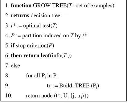
The decision trees are constructed in a top-down fashion by choosing the most appropriate attribute each time as shown in figure 1. An information-theoretic measure is used to evaluate features, which provides an indication of the “classification power” of each feature [4]. Decision tree induction is an algorithm that normally learns a high accuracy set of rules. Basically, given a data set, a node is created and a test t* is selected for that node. A test is a function from the example space to some finite domain. Typically the test for which the subsets of the partition are maximally homogeneous with respect to some target attribute (the “class”, for classification trees) is selected. For each subset Pj of the partition P induced by t*, the procedure is repeated and the created nodes become children of the current node. The procedure stops when stop criterion succeeds: this is typically the case when no good test can be found or when the data set is sufficiently homogeneous already.
Fig 1 A generic algorithm for top-down induction of decision trees
The algorithm computes the information gain of each attribute. The attribute with the highest information gain is chosen as the test attribute for the given set. A node is created and labeled with the attribute, branches are created for each value of the attribute, and the samples are partitioned accordingly
3. ISSUEINCLASSIFICATIONUSINGDECISIONTREEINDUCTION
Efficiency and scalability are fundamental issues concerning classification in large databases. The increasing computerization of all aspects of life has led to the storage of massive amounts of data. Large scale data mining applications involving complex decision making can access billions of bytes of data. Hence, the efficiency of such applications is paramount. The efficiency of existing decision tree algorithms, such as C4.5 and CART, has been well established for relatively small data sets [5].
Databases usually store large amounts of data in great detail. However, users often like to view sets of summarized data in concise, descriptive terms. Moreover, users like the ease and flexibility of having data sets described at different levels of granularity and from different angles.
In data mining application which contains the billions of records at low level are not useful to the users of the system to make meaningful decision. In such application the user are more interested in data at more abstract level to help them in decision making. It is nontrivial for users to determine which dimensions should be included in the analysis of classification. Data relations often contain 50 to 100 attributes, and a user may have little knowledge regarding which attributes or dimensions should be selected for effective data mining. A user may include too few attributes in the analysis, causing the resulting mined descriptions to be incomplete or incomprehensive. On the other hand, a user may introduce too many attributes for analysis (e.g., by indicating “in relevance to ", which includes all the attributes in the specified relations). [1] Hence, relevance analysis may be performed on the data with the aim of removing any irrelevant or redundant attributes from the learning process. In machine learning, this step is known as feature selection [2]. Including such attributes may otherwise slow down, and possibly mislead, the learning step. Ideally, the time spent on relevance analysis, when added to
1. function GROW TREE(T : set of examples)
2. returns decision tree:
3. t* := optimal test(T)
4. P := partition induced on T by t*
5. if stop criterion(P)
6. then return leaf(info(T ))
7. else
8. for all Pj in P:
9. trj := Build_TREE (Pj)
the time spent on learning from the resulting “reduced" feature subset, should be less than the time that would have been spent on learning from the original set of features. Hence, such analysis can help improve classification efficiency and scalability.
So there is a need to develop such a system which gives them data at desired level which give birth to the new research field in classification of large data stored in database
3.1 Attribute Oriented Induction
Applying attribute oriented induction prior to classification substantially reduces the computational complexity of this data intensive process .To controlled the degree of generalization; the following techniques are applied in sequences. First apply the attribute threshold control technique to generalize each attribute and then apply relation threshold control to future reduce the size of the generalized relation. If the number of distinct values of an attribute is less than or equal to this attribute threshold, then further generalization of the attribute is halted. If the number of tuples in a generalized relation is less than the generalize relation threshold, then future generalization is halted.
3.2 Relevance Analysis
Then we apply attribute relevance analysis to the generalized data obtained from attribute oriented induction. we are using Information gain measure for finding the irrelevant or redundant attributes from the generalized relation. This further reduces the size of the training data.
4. METHODOLOGY
We address the above issues regarding the classification of large databases by proposing a technique composed of the following steps: 1) Cleaning the data by handling the missing values. 2) Generation of Concept
Hierarchy for nominal and numerical attributes. 3) Attribute Oriented Induction is then applies, to compress the
training data. 4) Apply relevance analysis to generalized data , to remove irrelevant data attributes, thereby further compacting the training data, and 5) Decision tree Induction at multiple level, which combines the induction of decision trees with knowledge in concept hierarchies
Algorithm (Gen_DT):
Perform data classification using a pre specified classifying attribute on a relational database by integration of data cleaning, concept hierarchy generation, and attribute oriented induction and relevance analysis with a decision tree induction method.
Input.
1) A data classification task which specifies the set of relevant data and a classifying attribute in a relational database DB,
2) ATi, Atribute Threholds for attribute Ai.
3) An exception threshold e, and 4) A classification threshold c. Output.
Classification of the set of data and set of classification rules Method.
1. Data cleaning: Apply the method to fill in the missing values for the numerical and nominal attributes in a database.
2. Concept Hierarchy Generation: Generate the concept Hierarchy for numerical attribute. For categorical Attributes find the ordering and define the concept hierarchy for that.
3. Data collection: Collect the relevant set of data, in R0, by relational query processing.
4. Attribute Oriented Induction: Using the concept hierarchies, perform attribute oriented induction to generalize R0 to an intermediate level. The resultant relation is GR. The generalization level is controlled by
ATi threshold.
5. Relevance Analysis: Perform relevance analysis on the generalized data relation, GR. We have used information gain ratio because it biases the decision tree against considering attributes with a large number of distinct values. So it solves the drawback of information gain and calculated using following equation.
Let S be a set consisting of s data samples. Suppose the class label attribute has m distinct values defining m distinct classes, Ci (for i = 1; : : :;m). Let si be the number of samples of S in class Ci. The expected information
needed to classify a given sample is given by:
mi
i i
m
p
p
s
s
s
I
1
2 2
1
,
,...,
)
log
(
)
(
(1)
v j mj j mj js
s
I
s
s
s
A
E
1 1 1)
,...,
(
...
)
(
(2)The smaller the entropy value is, the greater the purity of the subset partitions. The encoding information that would be gained by branching on A is
)
(
)
,...,
,
(
)
(
A
I
s
1s
2s
E
A
Gain
m
(3) The gain ratio for the attribute is defined as followsGain Ratio (A) =
)
,...
,
(
)
(
21
S
S
mS
A
Gain
(4)
We rank the most relevant attributes for the given classification tack and retain N (Threshold value for Rank) number of attributes to train the model. The resulting data relation is RR.
6. Decision Tree Generation
(a) Given the generalized and relevant data relation, RR, compute the information gain for each candidate attribute using equation [1] to [3].
Select the candidate attribute which gives the maximum information gain as the decision or “test" attribute at this current level, and partition the current set of objects accordingly.
(b) For each subset created by the partitioning, repeat Step 6(a) to further classify data until either (1) all or a substantial proportion (no less than c, the classification threshold) of the objects are in one class, (2) no more attributes can be used for further classification, or (3) the percentage of objects in the subclass (with respect to the total number of training samples) is below e, the exception threshold.
7. Classification Rule Generation: Generate rules according to the decision tree.
5. EXPERIMENTALRESULT
In order to study the performance, we implemented and tested the algorithm. We also implemented two algorithms for generating the concept hierarchy and testing database. The performance of theclassification-based method is affected by several factors such as the number of records, the classification threshold, the number of attributes etc. In this section we will take a closer look at how these factors actually affect the performance in our experiments.
In our experiments we used mainly well-known data set from the UCI repository [7]. Table 1 summarizes shortly the main characteristics of the data set. More comprehensive description can be found from the referred sources.
Classification Problem:
Given a database D
{age,work_class,education,marital_status,occupation,race,sex,capital_gain,capital_los,hours_per_week,native_c ountry } of tuples ( items, records ) and a set of classes C = { income <= 50k , income > 50K }, the classification problem is to define a mapping f : D -> C where each tuple is assigned to one class.
Attribute Detail:
Number of Attributes: There are 4 continuous and 7 categorical attribute in the given dataset.
No Attribute Name Possible Values
1 Age 74
2 Work Class 8
3 Education 16
4 Material Status 7
5 Occupation 14
6 Race 5
7 Sex 2
8 Capital-gain 123
9 Capital-loss 99
10 Hours-per-Week 96
11 Native Country 42
There are total 48842 instances in a original database. The data is divided into two parts using holdout method. 1. Training Data: 32626 Instances
2. Testing Data: 16216 Instances Class Distribution:
Probability for the label '>50K’: 23.93%. Probability for the label '<=50K’: 76.07%
Following are Concept Hierarchy we have used for the given Problem. All hierarchies are of type Set Grouping Hierarchy.
Set Grouping Hierarchy for Age {17 – 35 } Young { 36 – 60 } Middle_Aged { 61 – 100 } Old
{Young, Middle_Aged, Old } all (Age) Set Grouping Hirerarchy for Capital_Gain
{0 – 25000} Low {26000 – 50000} Medium {51000 – 75000} High {76000 – 100000} Very High
{Low, Medium, High, Very High} all (Capital_Gain) Set Grouping Hierarchy fo Capital_Loss
{ 0 – 1000} Low { 1001 – 2000 } Medium { 2001 – 3000 } High { 3000 – 3001} VeryHigh
{ Low, Medium, High, VeryHigh} all (Capital_Gain) Set Grouping Hierarchy for Hours_Per_Week
{0 – 25 } Low ( 26- 50 } Medium { 51 – 75 } High { 76 – 100 } VeryHigh
{ Low, Medium, High, Very High} all (Capital_Gain) Set Grouping Hierarchy for Work_Class
{ Private, Self-emp-not-inc, Self-emp-inc } Private { Fedral-gov,Local-gov,State-gov } Goverement { Without-pay,Never-worked } Others
{ Private , Goverement , Others } all(Work_Class) Set Grouping Hierarchy for Education
{ 1st – 4th , 5th – 6th , 7th – 8th , 9th ,10th , 12th , Pre-school,Prof school,Some college } Undergraduate {Assoc-acdm, Assoc-voc, Bachelors, HS-grad } Graduate
{ Masters, Doctorate } Masters
{Undergraduate , Graduate , Masters } all(Education) Set Grouping Hierarchy for Marital_Status
{Married-AF-spouse, Married-civ-spouse,Married-spouse-absent } Married { Never-married } Unmarried
{ Divorced , Separated ,Winowed } Others
{Marreid , Unmarried , Others } all (Marital_Status) Set Grouping Hierarchy for Occupation
{Adm-clerical,Exec-managerial, Sales} Administrative
{Craft-repair, Farming-fishing, Handlers-cleaners, Machine-op-inspct, Priv-house-serv, Transport-moving } Skilled
{Other-service, Prof-specialty, Armed-Forces, Protective-serv } Others {Administrative , Skilled , Others } all(Occupation)
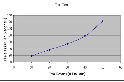
5.1 Scale up Performance
Time Taken
0 20 40 60 80 100 120 140
0 10 20 30 40 50 60
Total Records (In Thousand)
Ti
m
e
T
a
k
e
n
(In
S
e
c
o
n
d
s
)
Fig 2 Scale up Performance
Decision tree induction is used as a base classifier to classify the given datasets. We have measure the accuracy of different datasets using the decision tree and compared it with our proposed approach. Table 2 describes the accuracy comparison of both the methods. In almost every case we get the comparative accuracy in less time.
5.2 Performance Study on Different Classification Thresholds
Fig 3 shows the performance study we did for our Classification-based predictive modeling method on the same set of data but with different classification thresholds. In this experiment we wanted to learn how the different classification thresholds affect the performance of this algorithm with the request, all the other variables remaining the same. The classification thresholds we are using are 20%, 40%, 60%, 75%, 80%, 85%, 90%, 95% and 100%.
0 10 20 30 40 50 60 70 80 90 100
0 0.2 0.4 0.6 0.8 1 1.2
Classification Threshold
T
im
e
Ta
k
e
n (
In S
e
c
on
ds
)
Fig 3 Performance Study on Different Classification Thresholds
The experimental result is shown in Fig 3 which shows that with the increase in the classification threshold, the running time also increases because more and more nodes whose parent node cannot pass the increased classification threshold have to be constructed and information gain also has to be calculated at these nodes' parent nodes in order to select the next branching attribute. From Fig 3 we can also see that when the classification threshold is below a certain point. The time increase is also limited because in this testing scenario the numbers of nodes which can pass the lowest classification threshold but cannot pass this classification threshold are limited and thus the associated cost increase is limited.
5.3 Performance Study with Other Methods
0.79 0.795 0.8 0.805 0.81 0.815 0.82 0.825
Adaptive Bayes Network
Naive Bayes Support Vector Machine
Gen_DT
Algorithm
A
ccu
racy Accuracy
Fig 4 Comparison with other Methods
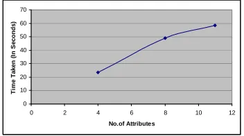
5.4. Performance Study on Different Numbers of Attributes
Figure 5 shows the performance study we did for our classification-based predictive modeling method on the same number of records but with different numbers of attributes. In this experiment we wanted to learn how different numbers of attributes affect the performance of this algorithm with a similar request, all the other variables being the same. The parameter values for our database are as follows:
Case 1: Number of attributes: 4 (including 3 descriptive attributes and 1 predictive attribute). The number of distinct values for each attribute is as following: 119 for first the descriptive attributes, 92 for second attribute , 7 for third attribute and 2 for the predictive attribute.
Case 2: Number of attributes: 8 (including 7 descriptive attributes and 1 predictive attribute). The number of distinct values for each attribute is as following: for first descriptive attributes, 92 for second attribute , 7 for third attribute , 73 for fourth attribute , 16 for fifth attribute , 2 for sixth attribute , 94 for seventh attribute and 2 for predictive attribute.
Case 3: Number of attributes: 11 (including 10 descriptive attributes and 1 predictive attribute). The number of distinct values for each attribute is as following: 119 for first descriptive attributes, 92 for second attribute , 7 for third attribute ,73 for fourth attribute , 16 for fifth attribute , 2 for sixth attribute , 94 for seventh attribute , 6 for eight attribute ,14 for ninth attribute , 5 for tenth attribute and 2 for predictive attribute.
0 10 20 30 40 50 60 70
0 2 4 6 8 10 12
No.of Attributes
Ti
m
e
Ta
k
e
n (
In S
e
c
ond
s
)
Fig 5 Performance Study on Different Numbers of Attributes
Figure 5 which show that with the increase in the number of attributes in the database the running time also increases primarily due to the increased overhead to select branching attribute at each node and constructing more nodes at additional levels in the constructed decision tree.
6. CONCLUSION
We have shown that when we apply Attribute Oriented Induction (AOI) to generalized the attributes and then apply relevance analysis to filter out some less relevant attributes before we constructs the decision tree, we get comparative accuracy in less time as compare to decision tree induction. Experimental result also shows that AOI and relevant analysis can improve the speed and possibly the accuracy of decision tree models build on datasets with a large number of attributes.
ACKNOWLEDGMENT
REFERENCES
[1] Petra Perner. Improving the Accuracy of Decision Tree Induction by Feature Pre-Selection. Applied Artificial Intelligence 2001, vol. 15, No. 8, p. 747-760.
[2] Dianhong Wang; Liangxiao Jiang (2007). “An Improved Attribute Selection Measure for Decision Tree Induction.”Fuzzy Systems and Knowledge Discovery, 2007. FSKD 2007. Fourth International Conference on Volume 4, Issue , 24-27 Aug. 2007.
[3] Hendrik Blockeel, Jan Struyf (2002) “Efficient Algorithms for Decision Tree Cross-validation”. Journal of Machine Learning Research 3 (2002) 621-650.
[4] Petra Perner, “Improving the accuracy of decision tree induction by feature preselection”, Applied Artificial Intelligence: An International Journal, 1087-6545, Volume 15, Issue 8, 2001, Pages 747 – 760.
[5] S Rasoul Safavian and David Landgrebe, “A Survey of Decision Tree Classifier Methodology”, IEEE Transactions on System, Man and Cybernetics, Vol.21 , No p. 660-674, May 1991.