A Novel Fast Hybrid Frequency Domain Approach For Evaluating Harmonic Power Flow In Electricity Networks

275

A Novel Fast Hybrid Frequency Domain

Approach for Evaluating Harmonic Power

Flow in Electricity Networks

Abstract: Ideally, an AC power supply should constantly provide a perfectly sinusoidal voltage signal at every customer location. Nowadays, many power electronic equipment are used in industry in seeking higher system reliability and efficiency, and more electronic or microprocessor controllers are used in power system to control AC/DC transmission lines or loads. Moreover, the importance of green energy such as wind and solar is continually growing in our societies not only due to environmental concerns but also to resolve the problem of access to electricity in rural areas. As a result of these issues, power quality problems especially generation of harmonics are on the rise in the distribution network. In electrical power system, harmonics have a number of undesirable effects on power system devices as well as on their operation. It therefore becomes imperative for power system engineers to analyze the penetration of harmonics from the various sources into the network which commonly is known as harmonic power flow evaluation. This paper proposed a novel fast hybrid frequency domain approach (FHA) to evaluate the steady state harmonic power flow with discrete harmonic frequency. The proposed method is applied to IEEE – 14 bus, IEEE New England 39 - bus, IEEE – 57 bus and IEEE 118 - bus power system respectively and compared with Newton – Raphson (NR) load flow method and Fast decoupled load flow method (FDLF) and the results validate the accuracy, robustness and authenticity of the proposed method..

Index Terms: Harmonics, IEEE test system, Load flow, Newton – Downhill method, Secant method. ————————————————————

1 INTRODUCTION

The ac electrical power systems should be designed not only for the sinusoidal voltages and currents but are expected to operate successfully for electronically switched and non - linear loads. Nowadays, the wide implementation of non – linear loads and power electronics devices in real power system such as switched mode power supplies, diode rectifiers, adjustable speed drives, compact fluorescent lamps, HVDC networks, thyristor – controlled reactors, static var compensators, electronic ballasts etc. introduces the considerable amount of harmonic currents into the system [1]. Utility companies are particularly concerned with harmonics as one of the major power quality problem since the presence of harmonics causes the deterioration of the power systems voltage and current waveforms, thus affecting the operation of electrical equipments and also polluting the electric distribution network [2]. The main effects of harmonic distortion of the voltage supply range from possible protective devices‘ nuisance tripping to interference with telephone communication circuits to increased equipment losses that significantly reduces the lifespan of equipment like transformers and cables and to failure of power factor correction capacitors [3]. From the power quality viewpoint, the restructured power market increases the penetration of FACTS controllers and inverter – based power generation units in the transmission activity. In addition, the increasing use of power switching devices at the consumer end worsens poor power quality scenarios [4].

Resonance identification, power system planning, equipment design, among other applications. Further, the related economic impacts of harmonics and electricity market liberalization have all established a need for evaluating harmonic power flow in electricity networks. Over the last decade, many approaches have been proposed and implemented by the researchers for evaluating the harmonic power flow [5]. According to the modelling techniques of power system components and non-linear loads, these approaches can be categorized into three categories: time domain, frequency domain and hybrid time-frequency domain methodologies. Despite the fact that time domain methods can accurately model system non – linearities (e.g. hysteresis and saturation), they require long computation time than frequency domain techniques especially for a large power system containing many non-linear loads with strong harmonic couplings. Hybrid time-frequency domain methods can achieve the benefits of the accuracy of the time domain and the simplicity of the frequency domain. However, the frequency domain methods are widely used. They represent static load flow with discrete frequencies. Also, they require less computation time compared to both time domain and hybrid time-frequency domain methods [6]. Newton-Raphson power flow method, a frequency domain technique, is mostly used to evaluate the harmonic power flow because of giving accurate results. However, it requires long computation time, and even leads to convergence problems for especially a large power system with many non-linear loads and strong harmonic couplings. Hence, several other methods such as decoupled and fast-decoupled harmonic power flow calculation methods are proposed and implemented to solve the problems [7]. However, these methods still encounter two problems: (1) iterative initial value must be close to the expected value, otherwise, the calculations may fail to converge, and (2) the Jacobian matrix should be calculated in each iteration, which may require longer computing time and make the calculation more complicated [8] In addition, the existing harmonic power flow calculation methods involve a single traditional harmonic source (e.g. six-pulse line-commutated __________________________

 Author is currently working as an Associate Professor at Department of Electrical Engineering, Nirma University, Ahmedabad, India. E-mail: pavan.ssdn@gmail.com

276 converters and arc furnaces) or single type of traditional

harmonic sources that includes only integer harmonics in small or medium single-phase power systems. However, with increasing use of renewable energy generations (e.g. WTs and PGs) and modern electric devices (e.g. EVCs), the power system contains several types of harmonic sources with a large frequency range, i.e. integer-harmonics, inter-harmonics and sub-inter-harmonics [9]. Therefore, a harmonic penetration evaluation method which can be applied to large power systems with multiple types of harmonic sources is required. With this motivation, the present paper proposed a novel fast hybrid frequency domain approach (FHA) to evaluate steady state harmonic power flow in single phase balanced power systems with discrete frequencies. Harmonic couplings are not considered in this proposed method and each harmonic injection current of harmonic source is assumed to be known. The term ―hybrid‖ represents that the proposed method incorporates three methods: the secant method, the Newton-Downhill method and the decoupled method. The proposed method is successfully tested on IEEE – 14 bus, IEEE New England 39 - bus, IEEE – 57 bus and IEEE 118 - bus power system respectively. The results of computing time, the number of iterations, fundamental and higher harmonic bus voltage magnitudes and the total harmonic voltage distortion are calculated and compared with Newton-Raphson method and the Fast decoupled load flow (DLF) method. The proposed algorithm reduces the number of iterations and solve the convergence problem successfully for all the test cases, thus validating its accuracy, robustness and authenticity as compared to the other load flow methods.

2

MATHEMATICAL

MODELLING OF

FAST

HYBRID

APPROACH

(FHA) FOR

HARMONIC

POWER

FLOW

EVALUATION

The performance of the proposed fast hybrid frequency domain method is illustrated in the block diagram shown in

Fig. 1.

As shown in figure 1, the inputs (two guess values) enter the secant method first in order to establish the initial values for the calculation at fundamental frequency. The proposed method combines the Newton-Downhill and the Decoupled method together to calculate the power flow at fundamental frequency thus reduces the calculation process and converge successfully. The initial values at higher harmonic frequencies are included in the calculation. An admittance-matrix based equation is used to calculate the harmonic penetration directly [10].

2.1 Secant Method

The secant method is a common and popular variation of the Newton-Raphson method for finding the roots of nonlinear equations. Compared to Newton-Raphson method that approximates the root with a tangent line, the Secant method uses secant lines (hence the need for two initial starting values) to calculate the root of a function f. It assumes a non-linear equationf(x) 0. f(x)is continuous

for interval [a, b]. Taking two initial assumptions of this interval, k1

x and xk(where k represents the number of

iteration) that makef(xk1)f(xk)0, and drawing a

straight line passing through (xk1,f(xk1)) and(xk,f(xk)),

the intersection, k1

x , between the straight line and the x –

axis is regarded as an approximate solution for the non – linear equation f(x)0 . However, if f(xk1)f(xk)0, the

secant method may not achieve an approximate solution. The secant line can be formulated by:

( ) ( ) ( )( )

1 1

k k

k k k

k _{x x}

x x

x f x f x f

y 

   

 

(1)

Let y = 0, then the horizontal ordinate at the intersection,xk1_{, is:}

( )

) 1 ( ) (

1

1 k

x f k x f k x f

k x k x k x k x

 

   

 _{k = 1, 2,..}

(2) The secant method can be explained geometrically as shown in Fig. 2.

) (x

f is a non – linear equation and it is continuous for

interval [a, b]. x*is the root of f(x)0. Assume xk1and k

x are two initial assumptions of interval [a, b]. If

0 ) ( ) (xk1 f xk 

f , as shown in blue, one draws a straight

line between (xk1,f(xk1)) and(xk,f(xk)), the intersection, 1



k

x , is an approximate solution. However, if

0 ) ( ) (xk1 f xk' 

f , as shown in red (figure 2), and drawing a

straight line passing through (xk1,f(xk1)) and(xk',f(xk')) such that there is no intersection between the straight line and x – axis, then, the method does not provide any solution.

Fig. 1. The performance block diagram of the proposed method (FHA)

277 2.2 Newton – Downhill Algorithm

Newton-Downhill algorithm, a method incorporating Downhill and Newton - Raphson approach, is an optimization algorithm that improves the convergence rate extending its convergence region and does not require initial iteration value calculation. Further, the Downhill algorithm requires less computing time and is more robust as compared to Newton – Raphson method [10, 11]. The Newton-Downhill algorithm introduces a downhill factor, 

, to make the iterative process monotonically decrease, that can be formulated by f(xk1) f(xk) (where k

represents the number of iterations), in order to improve the convergence and decrease the iterations. The traditional Newton – Raphson iterative approach can be mathematically expressed as:

) ( ' ) ( ) 1 ( k k k k x f x f x

x    (3)

where (k1)

x is the next iterative approximate solution and

k represents the number of iteration. The Newton – Raphson iterative approach after applying weighted average method is modified as:

xk1  x(k1)  (1 )xk

) ( ' ) ( k k k x f x f

x 

 (4)

where  is the downhill factor, and 0  1_{. Thus, the}

equation (4) is defined as the mathematical expression of Newton – Downhill algorithm. The downhill factor, , plays an important role in the Newton-Downhill algorithm as it expands the convergence scale and decreases the iterations. Hence, it is important to consider its value during the calculation. Normally, let  = 1 in the first

iteration, then the iterative approximate value xk1 is

achieved in accordance with equation(4). If

) ( )

(xk 1 f xk

f   , it moves to next iteration. Otherwise,

the downhill factor, , is halved andxk1is re-calculated

until the monotonic decrease of iterative process is satisfied. Although the monotonic condition,

) ( )

(xk 1 f xk

f   , may not achieved at the starting, as

long as  is small enough, it can be met.

2.3 Novel Fast Hybrid Harmonic Power Flow Evaluation Approach

The fast hybrid harmonic power flow calculation approach (FHA) is an improved iterative approach to calculate harmonic power flow in a power system. It uses the admittance-matrix-based equation to calculate the harmonic power flow directly at higher frequencies (h > 1), which is similar to the decoupled method. However, it makes improvements in the harmonic power flow evaluation at the fundamental frequency. It introduces the secant method to establish the iterative initial value in order to tackle the convergence problem caused by the poor initial value. It then combines the Newton-Downhill method and the Decoupled harmonic power flow

calculation approach to evaluate the harmonic penetration at fundamental frequency in power systems. It is proposed to make further efforts to solve the convergence problem and accelerate the calculation. The basic steps and procedure of the proposed fast hybrid harmonic power flow calculation approach (FHA) are explained as follows:

2.3.1 Computation of Iterative Initial Value:

The current balance for the fundamental frequency at each linear bus is shown in Fig. 3.

) 1 ( ,l r

I and

) 1 (

,l i

I represent the fundamental real and

imaginary line currents at the lth _{linear bus.} (1)

l

P and (1) l Q

denote the fundamental real and reactive powers at the

same bus. ~(1) *

      l

V is the conjugate value of the

fundamental bus voltage at bus l. The upper wave line of * ) 1 ( ~       l

V represents that it is a vector and the asterisk

means conjugate value. The subscripts r, i and l represent the real and imaginary parts and the bus number. The superscript (1) of all symbols represents the fundamental frequency. The fundamental current balance at each linear bus can be formulated as follow:

278 where l,…..,n represent the linear buses. The current

balance for both fundamental and harmonic frequencies at each non-linear bus is shown in Fig. 4.

Fig. 4. Current balance at a non – linear bus

where ( ) ,

h m r

I and ( )

,

h m i

I are the harmonic (including

fundamental frequency) real and reactive line currents at the mth _{non-linear bus.} ( )

,

h m r

g and ( )

,

h m i

g denote the harmonic

(including fundamental frequency) real and reactive non-linear load currents referred to the same bus. Note that the line and non-linear load currents are positive when they leave the non-linear bus. Therefore, the harmonic (including fundamental frequency) current balance at each non-linear bus can be expressed as below:

                                                      ) ( , ) ( , ) ( , ) ( , ) ( , ) ( , ) ( , ) ( , h n i h n r h m i h m r h n i h n r h m i h m r g g g g I I I I  

Now, the non – linear equation f(x) in equation 2 can be expressed as:

 

where subscript x of all symbols represents the bus number including both linear and non-linear buses k. 2.3.2 Computation of Harmonic Power Penetration After introducing the Newton-Downhill method to the decoupled harmonic power flow calculation approach, the mathematical equation used to evaluate the fundamental power flow is modified as [13]:

                                ) 1 ( ) 1 ( ) 1 ( ) 1 ( ) 1 ( ) 1 ( ) 1 ( ) 1 ( V L K N H Q P   (8)

Where ,V ,P and Q represent the voltage phase angle,

voltage magnitude, active and reactive power respectively.

L and K N

H, , are the four sub – matrices of Jacobian matrix.

 represents the downhill actor. The superscript (1) of all symbols represents the fundamental frequency. As the initial values of fundamental bus voltages

T n V V V _    

 (1) (1) 2

) 1 (

1 , ,..., are considered by the secant method,

the fundamental active and reactive power mismatches at each bus (except slack bus) can be calculated by:

          _  ) 1 ( ) , ( ) 1 ( ) , ( ) 1 ( ) , ( ) 1 ( ) , ( 1 ) 1 ( ) 1 ( ) 1 ( sin cos j i j i j i j i j j i SP i

i P V V G B

P   (9)

          _  ) 1 ( ) , ( ) 1 ( ) , ( ) 1 ( ) , ( ) 1 ( ) , ( 1 ) 1 ( ) 1 ( ) 1 ( sin cos j i j i j i j i n j j i SP i

i Q V V G B

Q   (10)

Where (1) ) , (i j

G and (1)

) , (i j

G represents the real and imaginary

part of fundamental line admittance between bus i and j

respectively. (1) ) , (i j

 represents the fundamental voltage

phase angle mismatch between bus i and j. Assuming the initial value of  = 1, the correction vectors _ (1)_and

) 1 (

V

 can be established by involving the calculated

fundamental active and reactive power mismatches in equation (8). The modified fundamental bus voltages can then be achieved. By putting these modified fundamental bus voltages into equations (9) and (10) respectively, the corresponding active and reactive power mismatches,

' ) 1 ( i P  and ' ) 1 ( i Q

 ,are calculated. If W(1)' W (1) (where

) 1 (

W represents the fundamental power mismatch vector,

T Q P     

 (1), (1) ), the downhill factor is halved. The above

procedure is repeated untilW (1)'  W (1) . After this, the

final modified fundamental bus voltages are regarded as the initial values for the next iteration of fundamental power flow calculation [12]. The iteration stops when the following convergence criterion for the fundamental power flow calculation is satisfied:

max ( , (1),..., (1), (1))

1 ) 1 (

1 Q Pn Qn

P (11)

Where  is given exiting circulation value (or a predefined tolerance) and is usually set to be 10-5 _{At higher}

frequencies, the harmonic power flow problem can be solved by using the admittance – matrix based equation directly as shown in equation (11)

_I(h) _Y(h)_V (h) ₍₁₂₎

279

3. HARMONIC SOURCES AND INITIAL VALUES

3.1 Harmonic Sources

Two six-pulse line commutated converters are considered as harmonic sources in the present study. The six-pulse converter is basically a polyphase converter and is widely used in household products. It generates more harmonic injection currents than the twelve and twenty four pulse converters [12]. Hence, the harmonic penetration could be significant. These two six-pulse converters are represented as six-pulse converter-1 and six-pulse converter - 2 respectively. The harmonic injection for each harmonic level (including the fundamental frequency) of both the six pulse converters is illustrated in Table 1 and 2 respectively. Further, it is mentioned that the highest harmonic order of both the converters is assumed as 29th_.

Table 1: Harmonic currents generated by the six pulse

converter – 1

Harmonic

Order ‘h’ Magnitude (p.u.)

Angle (in degree)

1 0.1 0

5 0.02 0

7 0.0143 0

11 0.0091 0

13 0.0077 0

17 0.0059 0

19 0.0053 0

23 0.0043 0

25 0.004 0

29 0.0034 0

Fig. 5. Flowchart of the proposed novel FHA algorithm

Table 2: Harmonic currents generated by the six pulse

converter – 2

Harmonic

Order ‘h’ Magnitude (p.u.) (in degree) Angle

1 1.000 0

5 0.0191 0

7 0.0131 0

11 0.0072 0

13 0.0056 0

17 0.0033 0

19 0.0024 0

23 0.0012 0

25 0.0008 0

29 0.0002 0

.2 Initial Values

The fundamental voltage magnitudes fluctuate around 1.0 p.u., while the harmonic voltage magnitudes are between 0.01 p.u. and 0.05 p.u. according to simulation experiments. Hence, it is assumed that the fundamental voltage magnitudes are 1.0 p.u. for all buses except the slack bus, since the fundamental voltage magnitude and phase angle of the slack bus are already known. Further, while the harmonic voltage magnitudes are assumed to take any desired value between 0.01 p.u. and 0.05 p.u., the phase angles in all harmonics (including fundamental frequency) are assumed to be 0 degrees for each bus except the slack bus. 0.50.0and 1.50.0in the interval [0.5, 1.5] are chosen to calculate the fundamental initial voltages of the linear load buses (i.e. PQ bus) and the non – linear load buses (i.e. PS bus) by the proposed method. It is necessary to consider the initial voltage magnitude for all higher order harmonics in the Newton-Raphson method. It is assumed that the initial value of each higher harmonic order is reduced by 0.01 p.u. than the previous value when the fundamental value is assumed 1.0 p.u. Also, the voltage phase angles for all higher harmonics are set to 0 degree.

4 IMPLEMENTATION OF THE PROPOSED ALGORITHM

280

Table 3: Location of harmonic sources for different IEEE

test cases

Sr. No. Test Case Harmonic Location of Sources

1 _System IEEE – 14 Bus Power _{Bus – 9} Bus – 5 and 2 _{Power System} IEEE New England 39 – Bus _{and Bus – 29} Bus – 23 3 _System IEEE – 57 Bus Power _{and Bus – 29} Bus – 15 4 _System IEEE – 118 Bus Power _{and Bus - 95} Bus – 22

< Insert Table -4 >

The variation of higher order harmonic voltage magnitudes (p.u.) at different nodes for all the considered test cases is illustrated in Fig. 6(a) – 6(d) so as to investigate and compare the variation of each harmonic order.

Fig. 6. Variation of higher order harmonic voltage magnitude (p.u.): (a) IEEE – 14 bus system (b) New England IEEE – 39 bus system, (c) IEEE – 57 bus system,

and (d) IEEE – 118 bus system

In order to investigate and compare the calculation accuracy of the proposed algorithm with other two methods (i.e. NR and FDLF method), the result differences between each method are illustrated and represented by the term ‗ERROR‘. The results achieved by the NR method are considered as the reference value because of its well-known accuracy. Moreover, it is implemented in MATLAB tool package which can be used directly. As a result, the values of ERROR_1 represent the result differences between the NR method and FDLF method. ERROR _2 represents the result differences between the NR method and the proposed FHA method. The maximum result differences of the fundamental bus voltage magnitude(V (1)), the total harmonic voltage distortion

(THDv), the total active and reactive powers at both sending and receiving ends (Ptotals, Ptotalr, Qtotals and Qtotalr),

and the total power loss on each branch (Ptotalloss) between

each method in different IEEE test power systems are (b) IEEE New England 39 – Bus System

281 summarized in Table 5 and the accuracy comparison in

terms of ERROR_1 and ERROR_2 is shown in Fig. 7 and Fig. 8.

< Insert Table 5>

(a) IEEE – 14 Bus System

(a) IEEE 118 – Bus System

Fig. 7. The result differences of the fundamental bus

voltage magnitude (p.u.): (a) IEEE – 14 bus system (b) New England IEEE – 39 bus system, (c) IEEE – 57 bus

system, and (d) IEEE – 118 bus system

(d) IEEE – 118 Bus System

(a) IEEE – 14 Bus System

282 (c) IEEE – 57 Bus Syste

FiThe result differences of active power flow at both sending and receiving end: (a) IEEE – 14 bus system (b) New England IEEE – 39 bus system, (c) IEEE – 57 bus system, and (d) and (e) IEEE – 118 bus system The simulation results and the accuracy comparison indicates that for all the IEEE test cases considered in the present paper, the proposed FHA algorithm has less number of iterations, less computation time, good convergence, and

thus has better accuracy and robustness compared with NR method and FDLF method.

5 CONCLUSIONS

In this paper, a novel fast hybrid method (FHM) that combines the secant method, the Newton-Downhill method and the decoupled method has been proposed and presented. The validation of the algorithm and comparative simulation results in four different IEEE test systems has been illustrated. Compared with NR method and FDLF method, the proposed method has less iteration numbers and computation time and provide high accuracy and better performance. Also, the NR method and FDLF method fail to converge when the initial bus voltage magnitude is 0.6 p.u. and 0.5 p.u. for all the four IEEE test systems considered in the present work. Moreover, the proposed FHM method is reliable in terms of convergence (i.e. converged successfully) as it used the secant method to establish the iterative initial value. In conclusion, the proposed FHM method can accomplish the harmonic power flow calculation both for small and large power systems effectively and with an acceptable level of accuracy.

R

[1] J. Arrillaga, B. C. Smith, N. R. Watson and A. R. Wood, ―Power System Harmonic Analysis‖, John Wiley and Sons, New York, NY, (1997).

[2] R. Dugan, M. F. McGranaghan and H. W. Beaty, ―Electric Power Systems Quality‖, McGraw-Hill Professional, United States of America, USA, (2002).

[3] M. Caserza Magro, A. Mariscotti and P. Pinceti, ―Definition of power quality indices for dc low voltage distribution networks,‖ in Instrumentation and Measurement Technology 2006 proceedings of the international conference in Sorrento, Italy, 2006, IEEE, USA, pp. 1885–1888, (2006).

[4] T. Ise, Y. Hayashi, K. Tsuji, ―Definitions of power quality levels and the simplest approach for unbundled power quality services‖, in Harmonics and Quality of Power, 2000 Proceedings of the ninth international conference in Orlando, USA, 2000, IEEE, USA, pp. 385–390, 2000.

[5] D. Xia, T.G. Heydt, ―Harmonic power flow studies part I - formulation and solution‖, IEEE Transactions on Power Apparatus and Systems, 101(1982) 1257– 1265.

[6] G. K. Singh, ―Power system harmonics research: a survey‖, European Transactions on Electrical Power, 19(2009) 151–172.

[7] W. M. Grady, S. Santoso, ―Understanding power system harmonics‖, IEEE Power Engineering Review, 21(2001) 8–

[8] M. Castilla, J. Miret, A, Camacho, J. Matas, L. De Vicuna, ―Reduction of current harmonic distortion in three-phase grid-connected photovoltaic inverters via resonant current control‖, IEEE Transactions on Industrial Electronics, 60(2013) 1464–1472.M. Aien, M. Fotuhi – Firuzabad, M. Rashidinejad, ―Probabilistic optimal power flow in correlated hybrid wind - photovoltaic power systems‖, IEEE Transactions on Smart Grid , (d) The result differences of active power at sending end for

an IEEE – 118 Bus System

283 1(2014) 130 – 138.

[9] M. Leonidopoulos, ―Fast Linear Method and convergence Improvement of Load Flow Solution Methods‖, Electric Power System Research, 16(1989) 23 -31.

[10]H. Yang, F. Wen, L. Wang, S. Singh, ―Newton-downhill algorithm for distribution power flow analysis‖, in Power and Energy Conference, 2008 Proceedings of the Second International

Conference PECon 2008, Johor Bahru, Malaysia, pp. 1628–1632, 2008.

[11]K.M. Hink, ―Harmonic mitigation of 12-pulse drives with unbalanced input line voltages‖, MTE Corporation, W147, No. 9525, 2002.

[12]J. M. Ortega, W. C. Rheinboldt, ―Iterative Solution of Nonlinear Equations in Several Variables‖, (Ed.) Beijing Academic Press, China, pp. 227-262, 1983.

Table 4: Number of iterations, CPU required time, time per iteration and results of Newton Raphson Method (NRM), Fast Decoupled Load Flow Method (FDLF) and Fast Hybrid Method (FHM)

Table 5: Summary of maximum result difference of each method.

IEEE – 14 Bus System New England IEEE – 39 _{Bus System} IEEE – 57 Bus System IEEE – 118 Bus System ERROR_1

(p.u.)

ERROR_2 (p.u.)

ERROR_1 (p.u.)

ERROR_2 (p.u.)

ERROR_1 (p.u.)

ERROR_2 (p.u.)

ERROR_1 (p.u.)

ERROR_2 (p.u.)

) 1 (

V 3.58e-6 3.58e-6 9.82e-7 9.82e-7 7.15e-6 7.15e-6 1.61e-5 1.61e-5

THDv 0.0012 0.0012 8.5e-6 8.5e-6 0.0044 0.0044 0.0033 0.0033

Ptotals -6.75e-5 -6.75e-5 -3.2e-5 -3.2e-5 -1.8e-5 -1.8e-5 -6.9e-5 -6.9e-5

Ptotalr -5.88e-5 -5.88e-5 -3.3e-5 -3.3e-5 -1.8e-5 -1.8e-5 -6.6e-5 -6.6e-5

Qtotals -9.81e-5 -9.81e-5 -5.6e-5 -5.6e-5 7.09e-5 7.09e-5 0.0001 0.0001

Qtotalr 0.0001 0.0001 -5.7e-5 -5.7e-5 7e-5 7e-5 9.65e-5 9.65e-5

284

APPENDIX – I

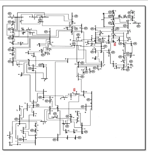
Figure I(a): Single line Diagram of IEEE – 14 Bus System

285