1st International Conference on Applied Soft Computing Techniques 22 & 23.04.2017
In association with
I
nternational
Journal of
Scientific
Research in
Science and
Technology
Data Partitioning Method for Mining Frequent Itemset Using MapReduce
R. Divya Bharathi1, A. S. Karthik Kannan2, E. Jai Vinitha3
1Department of IT, M.Tech, Mepco Schlenk Engineering College, Sivakasi, Tamilnadu, India [email protected]
2
Department of IT, Assistant Professor, Mepco Schlenk Engineering College, Sivakasi, Tamilnadu, India
3Department of IT, M.Tech, Mepco Schlenk Engineering College, Sivakasi, Tamilnadu, India
ABSTRACT
Existing parallel mining algorithm lacks in communication and mining overhead. To overcome this problem a data partitioning method using MapReduce model is proposed. In this model, three MapReduce tasks are implemented to improve the performance of frequent itemset mining in parallel. In second MapReduce job the mapper perform LSH based approach that integrates the item grouping and partitioning process. The reducer performs FP-Growth based on the partition data to generate all frequent patterns in the data. The main idea of data partitioning is to group relevant transactions and reduce the number of the relevant transaction. Extensive experiments using IBM Quest Market Basket Synthetic Datasets to show that data partitioning is efficient, robust and scalable on Hadoop.
Keywords : Frequent Itemset Mining, Mapreduce Model, Parallel Mining, Data Partitioning.
I.
INTRODUCTION
Frequent mining is an important problem in sequence mining and association rule mining. Increasing the speed of FIM is critical because Frequent itemset mining consumes more amount of mining time for its high computation in input and output process. When data in mining applications become very large, sequential frequent mining algorithm suffer from performance when it runs on single node [1] [2]. To overcome the problem of performance distortion therefore a framework using MapReduce a widely adopted programming model for processing big datasets by exploiting the parallelism among computing nodes of a cluster. We describe how to distribute a large dataset over the cluster to balance load across the Hadoop nodes to optimize the performance of parallel FIM.
The frequent itemset mining algorithm can be divided in to two Apriori and FP growth. Apriori is a well
known method for mining frequent itemsets in a transactional database. The algorithm works within a multiple pass generation and test framework, comprising the joining and pruning phases to reduce the number of candidates before scanning the database for support counting so each processor has to scan a database multiple times and to exchange an excessive number of candidate itemsets with other processors. Therefore Apriori parallel FIM solution suffer potential problems of high I/O and synchronization overhead, which make very difficult to scale up these parallel algorithm.
1.1 Motivations
The main contributions of this paper are given as follows
Volume 3 | Issue 4 | IJSRST/Conf/ICASCT/2017/25 1.2 MapReduce Framework
MapReduce is a promising parallel and scalable programming model for data intensive applications. A mapreduce program distributes computation as a sequence of parallel operations on dataset of key/value pairs. MapReduce has two phases namely, the map phase and Reduce phase. The map task splits the input in to a N number of fragments, which are distributed evenly to the first tasks across the cluster nodes by node manager for data processing. The input data is split in to small fragments as key-value pair and each map produces key-value pair as intermediate result. The reduce unit take the intermediate result of the map function as key and list of values and output the collection of values. Both tasks can be performed in parallel. The inputs pairs of map and the output pairs of reduce are managed by an underlying distributed file system. It offers automatic data management, transparent fault tolerant processing and highly scalable. The mapreduce can be an efficient platform for frequent itemset mining in large scale dataset.
Hadoop is open source implementation of mapreduce programming model which relies on its own Hadoop Distributed File System (HDFS). HDFS is designed for storing very large files with streaming data access patterns running on commodity hardware. At the heart of HDFS is a single Name Node a master server that manages the file system. The master node consists of task tracker, job tracker, name node and data node. A slave node acts as both a task tracker and data node.
II.
RELATED WORK
Many parallel algorithms have been proposed to enhance the performance of the Apriori frequent itemset mining. In Apriori based frequent itemset mining [3] they proposed three algorithms namely single pass counting (SPC), fixed passes combined counting (FPC) and Dynamic pass combined counting (DPC). SPC finds out frequent k itemset at k-th pass of database. FPC finds out (k-1) and (k+1) and up to (k+m) itemset in a map reduce phase. The third algorithm DPC, considers the workloads of nodes and
find out various length of frequent itemsets as possible in a map-reduce phase and also DPC calculates the candidate threshold and prevents the generation of many false positive candidates. It performs well when compared with the SPC and FPC.
X.Lin proposed Mr. Apriori [4] algorithm which runs on a parallel Map/Reduce framework. Prune (Ck+1) function to remove the non frequent itemset from the transaction. Where this function eliminates redundancy execution and ck cannot be subset of frequent item sets. This algorithm first calculate frequent itemset for each map node as the time complexity with respect to transaction t, Number of transactions n , Number of item in the transactions m. In second task is to calculate frequent item set with an additional item by joining, sorting and eliminating the duplicated items in each map node. Finally similarity can be calculated at the reduce nodes and eliminate the frequencies that do not meet the minimum support.
S. Hong, Z. Huaxuan, C.Shiping, and H.Chunyan [5] proposed improved FP growth algorithm which combines the sub-tree with same patterns which has high support count. Further it combines with mapreduce computing model MR-IFP (mapreduce-improved FP). It uses the depth first method to mine the frequent itemsets and saves a great deal of space. Built cloud platform to implement the IFP based on linked list Therefore it achieves high efficiency and scalability.
M. Liroz-Gistau, R. Akbarinia, D. Agrawal, E.Pacitti, and P. Valduriez [6] state that Map Reduce jobs are executed over distributed system composed of a name node and data nodes. Input is dividing into several splits and assigned to map tasks. MR-Part A partitioning technique is used for automatic partitioning of mapreduce input phase and a locality scheduling is done at the reduce tasks simultaneously so it reduce the amount of data shuffling between map unit and reduce unit .
Volume 3 | Issue 4 | IJSRST/Conf/ICASCT/2017/25 mapreduce to parallelize FP growth. First phase
divides entire mining task in to relatively even sub task to improve parallelization. The second phase divides all the load units in to several groups. It eliminates dependency between parallel tasks. In order to balance the load a work load of each mining unit is calculated and then fairly divides this unit into several groups. By using this balance metric BPFP achieves high parallelization.
III.
PROPOSED WORK
3.1 Partitioning of Data
Data partitioning is done using voronoi diagram based partitioning [8]. In this technique spaces are divided into number of parts. In prior a group of set which is referred as pivots (seeds) is chosen at preprocessing phase. For each pivot point there is a corresponding part consisting of all data points closer to it .The split regions for particular pivot are called voronoi cells. For a dataset D set of k pivots are selected then all objects in the Dataset D are partitioned into k disjoint sets (denoted as G1, G2,..Gk) and each object in D are assigned to the nearest pivot.
3.2 Distance Metric
In order to compute the similarity between the transactions Jaccard similarity is computed. A Jaccard similarity value 1 indicates two transactions are highly similar. The similarity between of two transactions T1 and T2 is given as below,
J (T1,T 2) =
J(T1,T2) is a value in between 0 to 1,if it is zero then row set is not equal, if it is 1 then the row set are same.
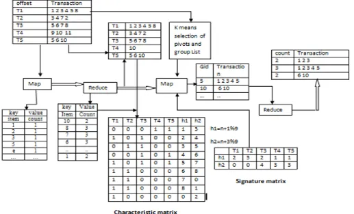
3.3 K-means selection of pivots
Pivot selection is the main process in partitioning the data. K-means strategy is used to select the pivots. It aims to partition m objects into k clusters. Given a set of objects (y1,y2…yk) are partitioned in to clusters
c1,c2,.ck where each data points belong to a cluster for a particular mean. Pivot selection is carried out preprocessing phase.
3.4 Partitioning Strategies
The two partition strategies are MinHash and LSH-Based partitioning in that MinHash is a basic foundation for Locality Sensitive Hashing.
3.4.1 MinHash
MinHash provides solution to determine the similarity between two sets [9]. MinHashing technique is mainly for dimension reduction large sets are replaced by smaller sets called “signatures”. There are two phases to generate signatures.
1) Characteristic matrix 2) MinHash Signatures
Characteristic matrix
Characteristic matrix will be obtained from FList (frequent one itemset List) and original dataset. Where column represent transaction and row denotes items in the transaction. For a given Dataset D= {T1, T2, .Tk}, which contains m items. If the item in the FList present in the transaction T1 then the item alone will be set as 1 otherwise it will be set as 0. Likewise the entire transaction in Dataset will be checked with FList and m (number of items) by n
(number of rows) characteristic matrix of M will be obtained.
3.4.2 MinHash Signatures
Volume 3 | Issue 4 | IJSRST/Conf/ICASCT/2017/25 columns but very less rows, thereby drastically
reducing the dimensions.
LSH-Based partitioning
Based on the banding technique, the rows in the signature matrix are divided into (b x r) where b represents the number of bands. Each band consists of maximum r rows. For each band a hash function is defined. The function takes column of its corresponding band and hashes them to large number of buckets. We can use the same hash function. For a any hash family if any two sets m1 and m2 satisfy the below conditions, then hash family is called (R, q, m1, m2).
A) If ||m1-m2|| < R B) If ||m1-m2|| < cR
Above condition is used to check similar sets are mapped in to the same buckets and dissimilar sets will be mapped in the individual bucket in hash table
IV.
IMPLEMENTATION
Data partitioning phase consist of three phases. In preprocessing phase selection of k pivots will
be done at the master node , which will be the input for second phase in mapreduce.
A. First MapReduce job
The first MapReduce phases discovers all frequent one-itemsets. The transaction in the dataset is partitioned into Data Nodes and items
in the
transaction and items in the transaction are
counted parallel.
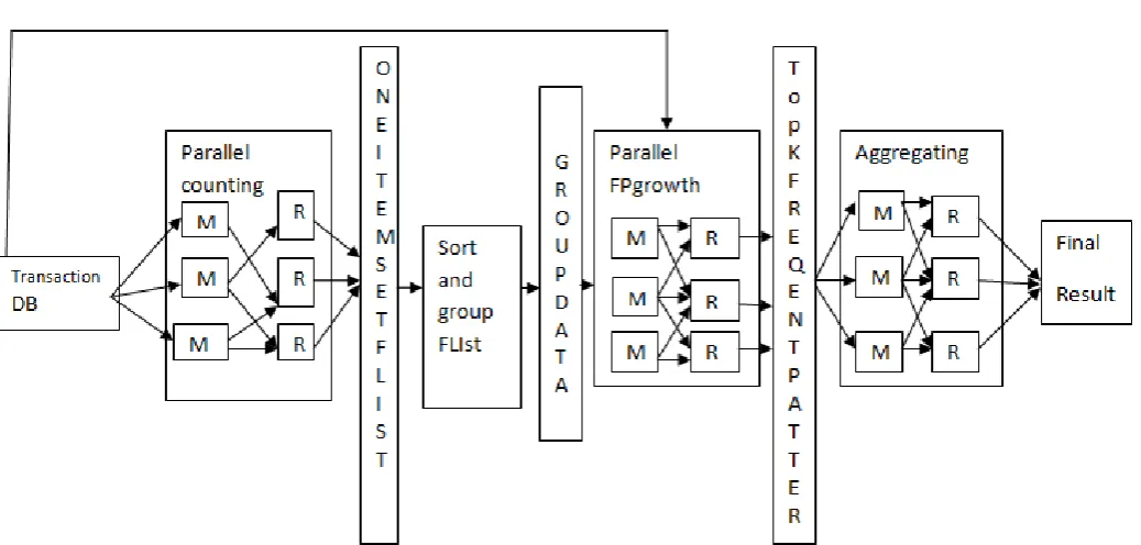
System Architecture
Volume 3 | Issue 4 | IJSRST/Conf/ICASCT/2017/25
Figure 2. Overview of Data Partitioning Algorithm
The input of Map tasks is a database, and the output of Reduce tasks is one frequent itemsets. The map input format will be <Long Writable offset, Text value> and the reduce output format will be in the format of <Text item, Long Writable count> then the frequent one itemset count along with itemsets are stored in a file called F-List.
B. Second MapReduce job
Mapper
First MapReduce output will be given as an input for the second phase in MapReduce. In second MapReduce phase sorting of frequent one itemset will be done using descending order and again it will be stored in a file F-List. By using this F-List signature matrix will be generated. Using k pivots similar transactions are grouped together and form a Group List with the corresponding unique group id (Gid). From the signature matrix LSH-Based partitioning is carried with corresponding Gid.
Reducer
Each reducer performs the local fp growth. Second mapreduce output will be used to generate frequent all patterns. fp growth while processing produce more dependent transactions are partition and it discovers the frequent transaction as final result.
C. Third MapReduce job
The last MapReduce job aggregates the result obtained from the second MapReduce job. Using the frequent pattern and generates candidate itemset for each itemsets and creates the final output.
Algorithm 1 LSH-fp-growth
Input: FList, k pivots, DBi;
Output: Transactions for each Group id
Volume 3 | Issue 4 | IJSRST/Conf/ICASCT/2017/25 2: load FrequentList(FList), m pivots;
3: Grouplist will be generated from the FList and m pivots
4: for each Transaction in Database perform 5: split the items in transaction and store it as
items[]
6: for every item in items[] perform
7: if items is present in FList then store the item in b[]
8: if end 9: for end
10: put the Generated-signature matrix(b[]) into arraylist of signaturematrix;
11: For end
12: For every ((column)i in signaturematrix) perform
13: divide column of the signaturematrix into B bands with r rows;
14: Store the column in Hashbucket using hashmap
15: For end
16: if one band of column in signaturematrix and pivot pk is mapped in to same bucket do 17: Assign j to the Gid;
18: Output contains Gid and new transaction tree of bi
19: If End
20: For each Grouplist (transaction≠i) do
21: if column in sigmatrix contains item in Grouplist then
22: Assign Gid to t;
23: Output contains Gid and new transaction tree of bi
24: If end 25: For end 26: Function end
Input: transactions corresponding to each Gid; Output: frequent k-itemsets
28: Reduce contains key as Groupid and values as database
29: Load Grouplists;
30: perform Grouplist according to Gid 31: perform local fp growth
32: for all (Transaction in Database Gid) do 33: build FP tree for the transaction
34: for end
35: for all element in b do
36: Define maxheap with the size K 37: perform TopKFpgrowth in maxheap 38: for all transaction in TopKFpgrowth
39: Output contains final transaction and support
40: for end 41: for end 42: function end
In LSH Algorithm each map phase takes transaction as pair <Long writable offset, Text record> then FList and k pivots are loaded initially. Each item in the transactions is split and compares with the FList items and stored in an array list b. From the b characteristic matrix and signature matrix will be generated. The signature matrix will be divide in to B bands each of which contains r rows (B x r= l). Then the column in the signature matrix are inserted in to the number of hash bucket if the sets are similar then it will be hashed to the same bucket. Assume that the similarity between two columns of signature matrix is d then they both transactions are considered similar. If a column in the signature matrix shares the similar bucket with a band B in pivot p then it will be denoted as a pair< pk, Ti>. Finally the map output will be a pair of < pk, Ti> and in reducer fp growth will be performed to generate frequent patterns.
ALGORITHM 2 Creation of SIGNATURE-MATRIX
Input: item transaction matrix of b[]; Output: generated signature matrix b[]
1: Function to generate signature matrix of b[] 2: For N number of hashfunction
3: Assign every value in MinHash to max integer;
4: For end
5: For each(j=0;j<numberOfhashfunction;j++) perform
6: For every element in the b[ ] perform
Volume 3 | Issue 4 | IJSRST/Conf/ICASCT/2017/25 8: Convert byte to hash of value and perform left
shift 24 <- bytetohash[1];
9: Convert byte to hash of value and perform left shift 16 <- bytetohash[2];
10: Convert byte to hash of value and perform left shift 8 <- bytetohash[3];
11: Convert byte to hash of value <-bytetohash[4]; 12: hashindex←hashfunction[j]*hash(bytesToHas
h);
13: if( minhashvalue[j] ) > hashindex then 14: minhashvalues[j]=hashindex;
15: if end 16: For end 17: For end 18: Function end
Algorithm 2 describes about the generation of signature matrix. It is really difficult to create signature matrix from the large characteristic matrix. In order to avoid the complexity Minwise Independent permutation technique [10] is used to speed up the process. So the high dimensional matrix will be reduced to low dimensional matrix and time complexity is greatly reduced.
V.
DATASET DESCRIPTION
We generated a synthentic dataset using IBM quest market-basket data generator [11], initially the average transaction is set as 8 after that vary the average transaction and number of items to meet the various need in the experiment. The characteristic of our dataset are described in Table1.
Table 1:DataSet
Average length
Item in
transaction
Average size of the transaction
8 1000 6.5B
10 4000 17.5B
40 10000 31.5B
60 10000 43.6B
85 10000 63.7B
VI.
Experimental Evaluation
We evaluate the performance of partitioning technique in Hadoop equipped with 1 name node and 8 data nodes. Each node has an Intel Pentium-4.3.0 GHz processor 256 MB main memory and runs on the Linux 2.3 OS, on which java JDK 1.7.0 and Hadoop 2.1 are installed. We use the default replication factor 3 as a hadoop configuration parameter.
VII.
PERFORMANCE EVALUATION
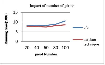
7.1 Impact of pivot Number
We vary the number of pivot point from 20 to 100 and obtain the running time. Our partition technique achieve overall performance when compared to pfp technique. if we increase pivot number then Running time get increased. When the pivot number is 60 the running time is minimized.
Figure 3. Impact of number of pivots
0 5 10 15
20 40 60 80 100
R
unni
ng
t
im
e
(100s
)
pivot Number
Impact of number of pivots
pfp
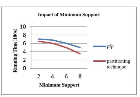
Volume 3 | Issue 4 | IJSRST/Conf/ICASCT/2017/25 7.2 Impact of minimum support count
Figure 4. Impact of minimum support count
VIII.
REFERENCE
[1] Yaling Xun, Jifu Zhang,Xiao Qin,” FiDoop-DP:Data Partitioning in frequent itemset mining on Hadoop Clusters IEEE Transcations on Parallel and distributed system, vol28, jan.2017.
[2] M. J. Zaki, “Parallel and distributed association
mining: A survey,” IEEE Concurrency, vol. 7, no. 4, pp. 14–25, Oct. 1999.
[3] Pramudiono and M. Kitsuregawa, “Fp-tax: Tree
structure based generalized association rule mining,” in Proc. 9th ACM SIGMOD Workshop Res. Issues Data Mining Knowl. Discovery, 2004, pp. 60–63.
[4] M.-Y. Lin, P.-Y. Lee, and S.-C. Hsueh,
“Apriori-based frequent itemset mining
algorithms on mapreduce,” in Proc. 6th Int. Conf. Ubiquitous Inform. Manag. Commun., 2012, pp. 76:1–76:8.
[5] X. Lin, “Mr-apriori: Association rules algorithm
based on mapreduce,” in Proc. IEEE 5th Int. Conf. Softw. Eng. Serv. Sci., 2014, pp. 141–144.
[6] S. Hong, Z. Huaxuan, C. Shiping, and H.
Chunyan, “The study of improved FP-growth algorithm in mapreduce,” in Proc. 1st Int.Workshop Cloud Comput. Inform. Security, 2013, pp. 250–253.
[7] M. Liroz-Gistau, R. Akbarinia, D. Agrawal, E.
Pacitti, and P. Valduriez, “Data partitioning for minimizing transferred data in mapreduce,” in
Proc. 6th Int. Conf. Data Manag. Cloud, Grid P2P Syst., 2013, pp. 1–12.
[8] L. Zhou, Z. Zhong, J. Chang, J. Li, J. Huang,
and S. Feng, “Balanced parallel FP-growth with mapreduce,” in Proc. IEEE Youth Conf. Inform. Comput. Telecommun., 2010, pp. 243–246.
[9] W. Lu, Y. Shen, S. Chen, and B. C. Ooi,
“Efficient processing of k nearest neighbor joins using mapreduce,” Proc. VLDB Endowment, vol. 5, no. 10, pp. 1016–1027, 2012.
[10] J. Leskovec, A. Rajaraman, and J. D. Ullman,
Mining Massive Datasets. Cambridge, U.K.: Cambridge Univ. Press, 2014.
[11] Z.Broder,M. Charikar,A. M. Frieze, and M.
Mitzenmacher, “Min-wise independent
permutations,” J. Comput. Syst. Sci., vol. 60, no. 3, pp. 630– 659, 2000.
[12] L. Christopher. (2001). Artool Project [J].[Online].Available
http://www.cs.umb.edu/laur/ARtool/ accessed Oct. 19, 2012
0 2 4 6 8 10
2 4 6 8
R
u
n
n
in
g
T
im
e(
1
0
0
s)
Minimum Support Impact of Minimum Support
pfp