Themed Section: Scienceand Technology
Automatic classification for NOAA- AVHRR Data using
k-means Algorithm
Adapa .Jyothirmai1, Dr. S. Narayana Reddy2, Dr. P. Jagadamba3
1Department of ECE, S.V.University College of Engineering, Tirupathi, Andhra Pradesh, India 2Professor of ECE, S.V.University College of Engineering, Tirupati, Andhra Pradesh, India
3Assistant Professor of ECE, Skit, Sri Kalahasthi, Tirupathi, Andhra Pradesh, India
ABSTRACT
This study proposes associate an automatic classification algorithm rule for NOAA(National Oceanic and Atmospheric Administration)-AVHRR (Advanced Very High-Resolution Radiometer) data It is well known that land cover conditions in the NOAA AVHRR data are classified into three different classes: ocean, land, and cloud. The algorithm consists of two major approaches: region of interest and classification algorithm. the region of interest extracted from the properties of the multispectral bands. k-means algorithm used detect the three classes. classification of image isn’t complete until an accuracy assessment has been conducted for the classified image. An accuracy assessment compares the information of two sources, i.e. pixels of the classified thematic map with reference image.
Keywords : Classification,K-Means, Accuracy Assignment
I.
INTRODUCTION
The AVHRR is a radiation-detection imager which will be used for remotely decisive bad weather and also the surface temperature. Note that the word surface will mean the surface of the Earth, the higher surfaces of clouds, or the surface of a body of water. This scanning radiometer uses 6 detectors that collect completely different bands of radiation wavelengths as shown below. The first AVHRR was a 4-channel radiometer, first carried on TIROS-N (launched October 1978). This was subsequently improved to a 5-channel instrument (AVHRR/2) that was in the beginning carried on NOAA-7 (launched June 1981). The latest instrument version is AVHRR/3, with 6 channels, first carried on NOAA-15 launched in May 1998. The AVHRR/3 instrument weighs approximately 72 pounds, measures 11.5 inches X 14.4 inches X 31.4
1.1.Extent of Coverage
The AVHRR sensor provides global (pole to pole) onboard collection of data from all spectral channels. Each pass of the satellite provides a 2399 km (1491 mi) wide swath. The satellite orbits the Earth half a day from 833 km (517 mi) above its surface.
1.2.Spatial Resolution
The average instantaneous field-of-view (IFOV) of 1.4 mill radians yields a LAC/HRPT ground resolution of approximately 1.1 km at the satellite nadir from the nominal orbit altitude of 833 km (517 mi).The GAC data are derived from an onboard sample averaging of the full (city areas, mountains, vegetation) resolution AVHRR data yielding 1.1-km by 4-km resolution at nadir. AVHRR data provide opportunities used for studying and monitoring vegetation conditions in ecosystems as well as forests, tundra, and grasslands. Applications consist of agricultural estimation, land cover mapping, producing image maps of large areas such as countries or continents and tracking regional and snow cove
II.
DATA AND LAND COVER INFORMATION
2.1. Land cover class
Based on the acquisition of NOAA AVHRR data, roughly classified into three classes: sea, cloud and land the proposed algorithm was used information of pure pixels for the classification of three classes
2.2. Properties of land cover class
The reference image acquired from combining three bands, i.e., band 1, band2 and band3 to obtain a color image. The different multispectral bands received at satellite receiver. information in a novel pixel in each band representedwith the DN numbers from 0 to 1023.converted to 8-bit data to reduce software implementations issues, easier visualization, no loss of information and less data for classification.
Properties of land cover classes
The histogram for band 2 data for classification of land covers classes
DNS of the cloud is high and its distribution is comparatively small
DNs of the sea is small and its distribution is small
The distribution of the DNs of the land is large; the land is found to be covered with complicated components barren soils).the DNs of the land is roughly found the range
Figure1.Three bands color composite image (band1,band2,and band3 are associated with blue,
green and red respectively.)
Figure 2.histogram of band 2
III.
METHODOLOGY
The flow process of the proposed method is as follows First consider the input image and then convert the image from RGB to HSV and processing can be done using k means clustering and followed by accuracy assignment.
3.1. Thresholding
Thresholding is that the simplest methodology of image segmentation from gray-scale.the thresholding method replaces every picture in a picture with a
black picture element. If the imaginary intensity is a smaller amount than some fixed firmly constant T, or a white image part intensity is larger than that constant .
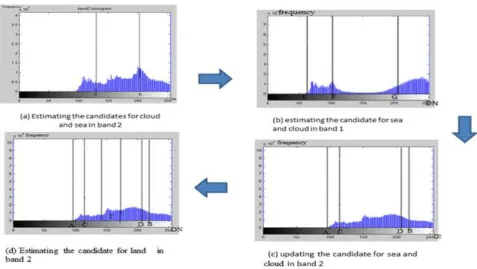
3.1.1. Estimation of sea and cloud candidate
Step 1: The thresholding of image based on a histogram of theimage. The range from 91 to peak value A in a low-intensity area on band 2 was assumed as the sea candidate. The range from peak value B in a high-intensity area to 255 was set as cloud candidate
Step 2: Two different ranges in band1, corresponds to a range from 90 to peak value A and to the range from peak value B to 255 in band2 were obtained respectively. The sea candidate in band1 is the range from E to point F(DN:60-105) and the cloud candidate is the range from point G to point DN:255.
Step 3: the ranges for the DNS in band 2, which belongs to the ranges of the candidates for sea and cloud in band 1 were obtained. Resulting ranges were combined candidates for sea and the cloud, respectively this facilitates the threshold of the sea candidate as the threshold c (DN:97) and the cloud candidate as the threshold D (DN:230) as shown fig 4(c) the sea candidate from (DN:60-102) and the from the threshold D to255 is the cloud candidate.
3.1.2. Estimation of land candidate
Land includes complicated components, the ranges of the land in each scene also changes with acquisition conditions By using thresholds of the sea and cloud candidate data obtained by The segmentation the above-mentioned process, the features value T was calculated by the equation (1).the range forT
was assumed to be a land candidate as shown fig 3(d).1
2
2
3
T
T
T
T
(1)T2 is the threshold of the sea candidate. After testing for suitable valu was set to 50
3.2. k-means Segmentation
The segmentation methodology is employed to extract the information from complex image. the main
objective segmentation is to extract that area of each region interest is spatially neighbours and therefore the pixels within the region are uniform with respect to a predefined basis.
Figure 3. Flow chart of estimating land cover classes sea and cloud in band 2
3.2.1.The k-means algorithm
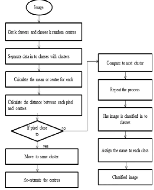
k-means is that the one of the learning algorithm method for clusters. Clusters the image is combination of the pixels in keeping with the some characteristics. In the k-means algorithm to start with we have to choose the number of clusters k. Then k-cluster centre are selected randomly. The distance between the each pixel to each cluster centres are measured. The distance may be of simple Euclidean function. Single pixel is compared to all cluster centres using the distance formula. The pixel is moved to particular cluster which has shortest distance between them. Then the centroid is re-estimated. Again each pixel is compared to all centroids. The process continues until the centre converges The improved k-means algorithm is a key to handle large scale data, which can select initial clustering centre determinedly to
assignments. With each following step, a data value can switch partitions, thus varying the values of the partitions at every step. k-means algorithms typically converge to a solution very quickly as opposed to other k-means algorithms have been. The first clusters the of the input image based on the RGB color of pixel information of each pixel, and the second clusters based on pixel intensity.
2 2
1 ( ) ( ) 1 ( ) 1
( ) || || || ||
2
k k
i j K i j
k c i c j k c i k
w c x x N x m
(2)For a given cluster assignment C of the data points, compute the cluster
For a current set of cluster means, assign each observation as:
2 1
( )c i arg min || k K ximk || (3)
Iterate above two steps until convergence
For a current set of cluster means, assign each observation
The distance between the cluster centres to each pixel is calculated as
. ( )
, 1,...,
K
r c i k
M K N
N
(4)
2
( ) arg min || i || , 1,...
D i x MK i N (5)
Repeat the above two steps until mean value convergence is obtained. The algorithm assumes that the data features form a vector space and tries to find normal clustering in them. As a part of this project, an iterative version of the algorithm was implemented. The algorithm takes a 2 dimensional image as input. There are always K clusters. There is always at least one item in each cluster. The clusters are non-hierarchical and they do not overlap. Every part of a cluster is closer to its cluster than any other cluster because closeness does not overlap
Figure 4. Flow chart of k-means algorithm
Every part of a cluster is closer to its cluster than any other cluster because closeness does not always occupy the ‘centre’ of clusters.
IV.
ACCURACY ASSIGNMENT
Classification of an image isn’t completed until an accuracy assessment has been conducted for the classified image. An accuracy assessment compares the information of two sources, i.e. pixels of the classified thematic map with Reference image. In alternate words, accuracy measures the agreement between a regular assumed to be correct and a classified image of unknown quality. Thus, accuracy assessment and error analysis permits quantitative comparisons and validate the classified data with the a particular data. It also helps in comparing the classification of remotely detected image being obtained through different classification techniques like supervised and unsupervised classifications or may be evaluated and assess supported by the image analyst.
4.1. Overall accuracy
To obtain overall accuracy of the classified image as compared to the reference image, calculate the diagonal elements of the matrix, represented by the Diagonal cells contain the total number of correctly identified pixels for each of the class that the image was classified interested in. Thus to get the overall accuracy (OA) The ratio of a sum of diagonal pixels by the total number of pixels. OA can be represented by the Equation 6
1
1 r i i
OA n
N
(6)where, N=total number of pixels, r= number of classes, n= correctly identified pixels in each class
4.2. Classification errors
The errors in the classified image, as the name suggests refers to the pixels which are not correctly classified as same class in the reference image and the classified image. There are two types of errors: underestimation, that is producer accuracy and overestimation that is user accuracy.
4.2.1. Producer Accuracy
The Producer's accuracy (PA), defined as the ratio of the number of pixels correctly classified in a particular class as a percentage of the total number of pixels belongs to that class in the reference image. PA can be represented by equation 6
i
icol
n PA
n
(7)
Where, ni = correctly identified pixels in the class and nicol= Column total for the considered class
4.2.2. User Accuracy
The user accuracy defined as to which is the percentage of the correctly identified pixels of a class to the total number of pixels allotted to the given class. UA can be represented by Equation 8
irow
ni UA
n
(8)
Where, ni = correctly identified pixels with in the class and nirow= Row total for the considered class
4.3. Kappa Coefficient, k
The accuracies of classified image are correct even for a absolutely random assignment of pixels to classes and can offer with the high percentage of accuracy values for the built an error matrix. Thus, Kappa coefficient another method, which is used as an accuracy indicator. The kappa coefficient method is a measure of the ratio between the reference image and the used classifier and the chance agreement between the reference image and a random classifier. Thus, with this piece of data obtained from a study of
a large quantity of numerical data. we are able to
detected image. Kappa coefficient is represented by Equation 4.
1 1
2
1
(
)
ˆ
(
)
r r
ii i i
i i
r
i i
i
N
x
x
x
k
N
x
x
(9)where, N=total number of samples, r= number of classes, xii= diagonal values in the matrix,
x i+ =total samples in row i, x+i=total samples in column i.
V.
RESULTS AND DISCUSSION
Figure 5.Thresholding image
The classification result obtained by a k-means by choosing three clusters and random points. The land, sea and cloud are classified clearly from the reference image through the conditions in the NOAA AVHRR data.
Figure 6.Thematic map of produced by k-means Algorithm classification. Blue indicates water and white indicates clouds. Brown indicates land area.
Figure 7. Thematic map of produced by k-means Algorithm classification. Blue indicates water and white indicates clouds. Brown indicates land area.
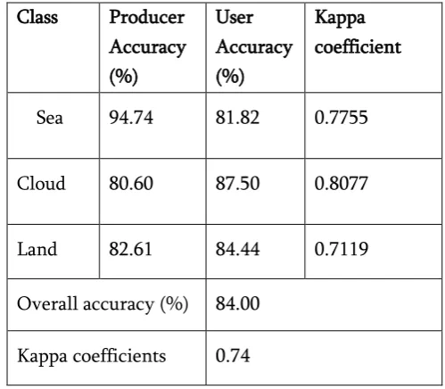
5.1. Accuracy Assignment
Validation of the results has been carried out by visual interpretation of reference image, sampling 100 validation points corresponding to the observation classified image. Positive samples were drawn from areas with clearly visible active sea, cloud and land. Negative sampling is necessary to assess the uncertainty of areas which were erroneously classified as active sea, cloud and land.
Table 1.Accuracy assignment for thematic map Class Producer
Accuracy (%)
User Accuracy (%)
Kappa coefficient
Sea 94.74 81.82 0.7755
Cloud 80.60 87.50 0.8077
Land 82.61 84.44 0.7119
Overall accuracy (%) 84.00
Table 2.Accuracy Assignment thematic map 2 class Producer
Accuracy (%)
User Accuracy (%)
Kappa coefficient
Sea 71.43 89.55 0.8955
Cloud 88.89 88.89 0.7980
Land 98.55 66.67 0.5833
Overall accuracy(%) 85.00
Kappa coefficients 0.7692
VI.
CONCLUSION
In this study, k-means clustering methods are developed to detect sea, land and cloud regions. The efficiency of the methods in identifying the region is tested visually. Experimental results prove to be better and yield better performance. Using the above techniques, valid and accurate results are obtained
VII.
REFERENCES
[1]. Cao, C. et al. 2008. Assessing the consistency of AVHRR and MODIS L1B reflectance for generating Fundamental Climate Data Records. Journal of Geophysical Research. Vol. 113. D09114. doi: 10.1029/2007JD009363.
[2]. Halthore, R. et al. 2008. Role of Aerosol Absorption in Satellite Sensor Calibration. IEEE Geoscience and Remote Sensing Letters. Vol. 5. pp. 157-161.
[3]. Heidinger, A. K. et al. 2002. Using Moderate Resolution Imaging Spectrometer (MODIS) to calibrate Advanced Very High-Resolution Radiometer reflectance channels. Journal of Geophysical Research. Vol. 107. doi: 10.1029/2001JD002035.
[4]. J. B. MacQueen (1967): "Some Methods for classification and Analysis of Multivariate Observations, Proceedings of 5-the Berkeley Symposium on Mathematical Statistics and Probability", Berkeley, University of California Press, 1:281-297
[5]. J. C. D. M. Esquerdo, J. F. G. Antunes, D. G. Baldwin, W. J. Emery, and J. ZulloJr, "An automatic system for avhrr land surface product generation," International Journal of Remote Sensing, vol. 27, pp. 3925-3942, 2006.
[6]. D. J. Berndt and J. Clifford, "Using dynamic time warping to find patterns in time series," in Proceedings of the Knowledge Discovery in Databases - KDD Workshop (KDD’1994), Seattle, Washington, USA, 1994, pp. 359- 370, ACM Press..
[7]. Kidwell, Katherine B., comp. and ed., 1995, NOAA Polar Orbiter Data (TIROS-N, NOAA-6, NOAA-7, NOAA-8, NOAA-9, NOAA-10, NOAA-11, NOAA-12, and NOAA-14) Users Guide : Washington, D.C., NOAA/NESDIS. [8]. Harris, J. W. and Stocker, H. "Maximum
Likelihood Method." §21.10.4 in Handbook of Mathematics and Computational Science.New York: Springer-Verlag, p. 824, 1998.
[9]. Hoel, P. G. Introduction to Mathematical Statistics, 3rd ed. New York: Wiley, p. 57, 1962. [10]. Press, W. H.; Flannery, B. P.; Teukolsky, S. A.;