data to ground-based data and its application to ACOS-GOSAT and TCCON

www.atmos-meas-tech.net/7/2631/2014/ doi:10.5194/amt-7-2631-2014

© Author(s) 2014. CC Attribution 3.0 License.

A method for colocating satellite

X

CO

data to ground-based data

and its application to ACOS-GOSAT and TCCON

H. Nguyen1, G. Osterman1, D. Wunch2, C. O’Dell3, L. Mandrake1, P. Wennberg2, B. Fisher1, and R. Castano1 1_{Jet Propulsion Laboratory, California Institute of Technology, Pasadena, CA, USA}

2_{California Institute of Technology, Pasadena, CA, USA} 3_{Colorado State University, Fort Collins, CO, USA}

Correspondence to: H. Nguyen ([email protected])

Received: 15 January 2014 – Published in Atmos. Meas. Tech. Discuss.: 14 February 2014 Revised: 25 June 2014 – Accepted: 30 June 2014 – Published: 19 August 2014

Abstract. Satellite measurements are often compared with higher-precision ground-based measurements as part of val-idation efforts. The satellite soundings are rarely perfectly coincident in space and time with the ground-based measure-ments, so a colocation methodology is needed to aggregate “nearby” soundings into what the instrument would have seen at the location and time of interest. We are particularly interested in validation efforts for satellite-retrieved total col-umn carbon dioxide (XCO₂), whereXCO₂ data from Green-house Gas Observing Satellite (GOSAT) retrievals (ACOS, NIES, RemoteC, PPDF, etc.) or SCanning Imaging Absorp-tion SpectroMeter for Atmospheric CHartographY (SCIA-MACHY) are often colocated and compared to ground-based columnXCO2 measurement from Total Carbon Column

Ob-serving Network (TCCON).

Current colocation methodologies for comparing satel-lite measurements of total column dry-air mole fractions of CO2 (XCO2) with ground-based measurements typically

involve locating and averaging the satellite measurements within a latitudinal, longitudinal, and temporal window. We examine a geostatistical colocation methodology that takes a weighted average of satellite observations depending on the “distance” of each observation from a ground-based location of interest. The “distance” function that we use is a mod-ified Euclidian distance with respect to latitude, longitude, time, and midtropospheric temperature at 700 hPa. We apply this methodology toXCO₂retrieved from GOSAT spectra by the ACOS team, cross-validate the results to TCCONXCO2

ground-based data, and present some comparisons between our methodology and standard existing colocation methods showing that, in general, geostatistical colocation produces smaller mean-squared error.

1 Introduction

Carbon dioxide (CO2) is an important anthropogenic green-house gas, and quantifying the exchange of CO2between the atmosphere and the Earth’s surface is a critical part of the global carbon cycle and an important determinant of future climate (Gruber et al., 2009). One important measure of CO2 is total column carbon dioxide (XCO₂), which is available from ground-based Total Carbon Column Observing Net-work (TCCON; Wunch et al., 2011a) and from space-based satellite instruments such as the Greenhouse gases Observ-ing Satellite (GOSAT; Yokota et al., 2004; Hamazaki et al., 2005) and the SCanning Imaging Absorption SpectroMe-ter for Atmospheric CHartographY (SCIAMACHY; Bovens-mann et al., 1999).

understanding of the instrument’s calibration, uncertainties in the O2and CO2 absorption cross sections, and subtle er-rors in the implementation of the retrieval algorithm (Crisp et al., 2012).

Often, there are spatial and temporal mismatches in the observed locations of the remote sensing instrument and ground-based validation instrument, and some spatial (and temporal) interpolation is required in order to “colocate” the two sources of data before a direct comparison is possible. We define “validation colocation” as estimating, through in-terpolation using nearby satellite observations, what a remote sensing instrument would have seen at a certain chosen loca-tion and time. In this paper, we examine a new colocaloca-tion methodology that is mathematically motivated in an error-minimization framework. Specifically, we are interested in developing a colocation methodology to combine retrieved XCO₂data from GOSAT spectra using the Atmospheric CO2 Observations from Space (ACOS) for comparison against TCCONXCO2data with the goal of minimizing the expected

interpolation error.

Colocation methods forXCO2 in the existing literature

in-clude geographical,T700(Wunch et al., 2011b), and model-based (Guerlet et al., 2013) colocation. Geographical coloca-tion typically defines a spatiotemporal neighborhood region, also known as a coincidence criterion, around the location of interest and then take summary statistics (e.g., mean or me-dian). Examples of geographical colocation includes averag-ing all same-day satellite observations fallaverag-ing within±5◦of a location of interest (Inoue et al., 2013), averaging all ob-servations falling within 5◦ and±2 h (Cogan et al., 2012), and taking the monthly median of all observations within a 10◦_×10◦_{lat–long box (Reuter et al., 2013).}

More sophisticated colocation methodologies add other correlated geophysical covariates in constructing such “neighborhoods” under the principle that conditioning on these additional correlated covariates would improve the quality of the comparison. Wunch et al. (2011b)’sT700 colo-cation method takes the average of all GOSAT observations falling within±30◦longitude,±10◦latitude,±5 days, and

±2 kelvin inT700of the TCCON location of interest. Guer-let et al.’s model-based method similarly takes the average of all same-day satellite values that fall within ±7.5◦latitude,

±25◦longitude, and±0.5 ppm of the 3-day-averaged model XCO₂data.

All the colocation methodologies above operate on an im-plicit assumption that observations “near” one another are more likely to be correlated, where “nearby” indicates be-ing proximal in a coordinate space and metric. The notion of “nearness” is captured in the definition of “neighborhood” that they specify; however, all observations falling within such a neighborhood are given equal weights in the compu-tation of the summary statistics. While this approach might be intuitive and straightforward, it fails to take further ad-vantage of the spatial information encoded within the coinci-dent locations. For instance, suppose that we have 10 satellite

observations falling within a coincident neighborhood of a ground-based station. The colocation methods above do not distinguish between the case where we have 10 satellite ob-servations retrieved exactly at the ground-based station and the case where the 10 observations are retrieved far away on the edge of the neighborhood region; the colocation methods would return the same colocated value in both cases.

In this paper, we present a refinement of these coloca-tion methodology by modeling the correlacoloca-tion structure as a function of “distance” using geostatistics, and then weight-ing nearby satellite observations by their correlation with one another and correlation with the location of interest. Our geostatistical methodology is motivated under an error-minimization mathematical framework and is related to op-timal interpolation (for more detail, see kriging in Cressie, 1993, Chapter 2). Our methodology has the same framework as Zeng et al. (2014), although they applied the methodology in the context of gap-filling CO2from regional data and not for defining colocation criteria, and they did not consider the addition of non-spatial and non-temporal covariates in their model.

The benefits of a geostatistical approach include explicit specification of the underlying covariance structure, error propagation, and minimized expected mean-squared error. All colocation methodologies are essentially interpolation techniques, which result in an interpolation uncertainty that is incorporated into the variability of the colocated/validation data comparison. It is important to minimize the interpolation error so that we can better assess the underlying variability and bias between the satellite and validation data. The geo-statistical colocation methodology has the attractive theoret-ical property that, given the correct spatial correlation struc-ture, it has the lowest interpolation error of all linear method-ologies.

In Sect. 2, we describe the data from ACOS-GOSAT and TCCON. Section 3 contains the details of our methodology as well as the estimation procedure, and we compare the per-formance of our geostatistical methodology to existing colo-cation methods in Sect. 4. Summary and discussion of the methodology along with possible extensions are presented in Sect. 5.

2 Overview of ACOS-GOSAT, TCCON, and auxiliary data sources

altitude, and it completes an orbit every 100 min. The satel-lite returns to the same observation location every 3 days (Morino et al., 2011).

Following the failure of the Orbiting Carbon Observatory (OCO) launch in February 2009, the OCO project formed the Atmospheric CO2Observations from Space (ACOS) task and, under agreement with NIES, JAXA, and MOE, applied the OCO retrieval algorithm to the GOSAT spectra to com-pute column-averaged dry-air mole fractions of CO2. The ACOS-GOSAT data processing algorithm is based on the op-timal estimation approach of Rodgers (2000) and is described in detail in O’Dell et al. (2012). It is modified from the OCO retrieval algorithm (Bosch et al., 2006; Connor et al., 2008; Boesch et al., 2011) to account for the different physical viewing geometries and properties such as instrument line shapes and noise models.

In this paper, we assess the performance of different cation methods on ACOS-GOSAT data by comparing colo-cated values to the more precise and accurate TCCON data. We use the v3.3 release of ACOS-GOSAT data, available from the Goddard Data and Information Services Center spanning July 2009 to April 2013 (see ACOS Data Access in the References for notes). GOSAT data are divided into three categories: glint (ocean) data, land high (H)-gain data, and land medium (M)-gain data. The v3.3 data user’s guide notes that M-gain data and ocean glint data have some de-ficiencies in that particular version and should only be used with heightened caution (Osterman et al., 2013). Hence in this paper we only make use of H-gain land data.

Following the recommendation of the data user’s guide, we screen the v3.3 H-gain data using a set of 11 criteria to obtain data suitable for scientific analysis. The set of screen-ing criteria is reproduced in Table 5. The ACOS-GOSAT data have a bias that is known to be correlated with certain other variables such as air mass, blended albedo, and posterior– prior surface pressure difference (Wunch et al., 2011b). The v3.3 data user’s guide recommends a linear bias correction to ACOS-GOSATXCO2based on the difference between the

retrieved and prior surface pressure from the A-band cloud screen and the ratio of the signal in the strong CO2band to that of the O2A band (Osterman et al., 2013). However, since such bias correction was done through comparison of v3.3 ACOS retrievals with models and TCCON retrievals, we re-frain from applying the v3.3 bias correction to avoid potential “feedback” in the comparison of our colocated v3.3 ACOS and TCCON values.

TCCON consists of ground-based Fourier transform spec-trometers that record direct solar spectra in the near in-frared. These spectra are then used to retrieve column-averaged abundances of atmospheric constituents, includ-ing CO2, CH4, N2O, HF, CO, and H2O, which are directly comparable with the near-infrared total-column measure-ments from space-based instrumeasure-ments (Wunch et al., 2011a). Whereas GOSAT retrievals are susceptible to variability re-sulting from contamination by optically thick clouds and

aerosols that were missed by the cloud-screening process (O’Dell et al., 2012), TCCON directly observes the solar disk and hence is less sensitive to errors from scattered light (Crisp et al., 2012).

TCCON sites sample in a diverse range of atmospheric states, which include tropical and polar regions, continental and maritime, polluted and clean, providing valuable vali-dation link between space-based measurements and the ex-tensive ground-based in situ network (Wunch et al., 2011a). TCCONXCO2 data in turn are validated against integrated

aircraft profiles (Washenfelder et al., 2006; Deutscher et al., 2010; Messerschmidt et al., 2011; Wunch et al., 2010) and have a precision and accuracy of∼0.8 ppm (Wunch et al., 2010).

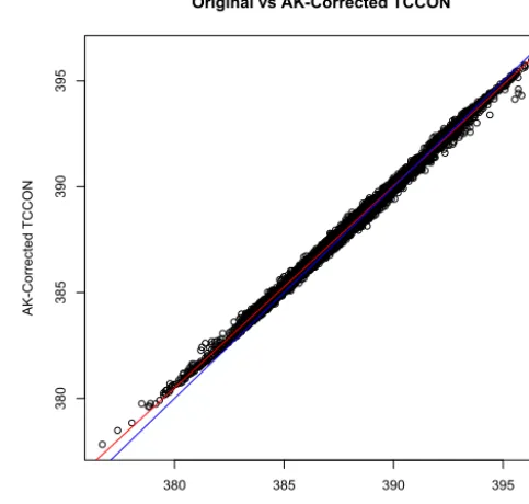
We use the 2012 release version of the TCCON data (“GGG2012”) from the TCCON Data Archive (see TCCON Data Access in the References for more information) for the following 16 locations: Bialystok, Bremen, Darwin, Eureka, Garmisch, Izaña, Karlsruhe, Lamont, Lauder (both 120HR and 125HR), Ny-Ålesund, Orleans, Park Falls, Reunion, So-dankyla, Tsukuba (both 120HR and 125HR), and Wollon-gong. At each TCCON location, we use all available data that fall within the period of July 2009 to April 2013. A map of the TCCON locations is shown in Fig. 1. This particu-lar version of TCCON data suffered from site-to-site biases due to a laser sampling issue inside the Bruker 125HR in-struments, and thus we corrected for these biases using the TCCON recommended bias corrections (for more detail, see TCCON Data Access, 2013).

Atmospheric variability ofXCO₂has been shown to be cor-related to the free-tropospheric potential temperature, which can be considered as a proxy for equivalent latitude forXCO₂ in the Northern Hemisphere (Keppel-Aleks et al., 2011). In this paper, we follow Wunch et al. (2011b) in making use of midtropospheric temperature as one of the covariates along with latitude, longitude, and time. Specifically, we use the midtropospheric temperature field at 700 hPa from the National Centers for Environmental Prediction and the Na-tional Center for Atmospheric Research (NCEP/NCAR) re-analysis product, which uses a frozen state-of-the-art analy-sis/forecast system and performs data assimilation using past data (Kalnay et al., 1996). The midtropospheric temperature field at 700 hPa should be directly proportional to the poten-tial temperature at 700 hPa for the range of temperature of interest, and its inclusion as a covariate should allow us to construct better colocation metrics.

2.1 Averaging kernel correction

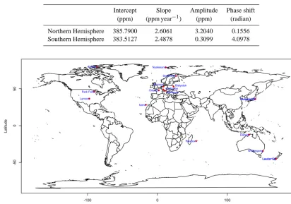
Table 1. Annual and seasonal trend coefficients.

Intercept Slope Amplitude Phase shift (ppm) (ppm year−1) (ppm) (radian) Northern Hemisphere 385.7900 2.6061 3.2040 0.1556 Southern Hemisphere 383.5127 2.4878 0.3099 4.0978

-100 0 100 200

-5

0

0

50

Longitude

Latitude

Bialystok Bremen

Darwin Eureka

Garmisch

Izana

Karlsruhe

Lamont

Lauder120

Lauder125

Nyalesund

Orleans Park Falls

Reunion Sodankyla

Tsukuba120 Tsukuba125

Wollongong

Figure 1. Map showing the 16 TCCON locations for which we perform GOSAT/ACOS and TCCON colocation comparison.

comparison is given in Sect. 4 and Appendix A of Wunch et al. (2011b).

Typically, to compare retrieval results from two different instruments with different viewing geometrics, retrieval al-gorithms, a priori profiles (xa), and averaging kernel (A), we need an common ensemble profile (xc) and covariance ma-trix (Sc); these represent the mean and variability of the at-mosphere at the common comparison location. As an alterna-tive, we can use one observing system to try to retrieve what the other system would have produced as its retrieved total column (Rodgers and Connor, 2003). Given that TCCON re-trievals are considered more precise and accurate, we smooth the TCCON value with the ACOS-GOSAT column averag-ing kernels to produce what ACOS-GOSAT would have pro-duced at the TCCON location given the TCCON profile as “truth”.

Fortunately, ACOS v3.3 a priori profiles and TCCON a priori profiles are very similar to one another, and hence we only need to account for differences in the averaging ker-nels. We use the following averaging kernel equation from Appendix A of Wunch et al. (2011b):

ˆ

z12=za+(γ−1)X

j

hja1jxaj, (1)

where za is the a priori XCO2; zˆi is the retrieved XCO2,

withi=1 for ACOS andi=2 for TCCON;his theXCO2

pressure weighting function; and a is the XCO2 averaging

kernel norm. The termγ is a scaling factor that produces the best fit of the TCCON output to the spectrum, and it is approximated as a ratio between the retrieved TCCONXCO2

and the a prioriXCO2,

γ≈z2ˆ

za .

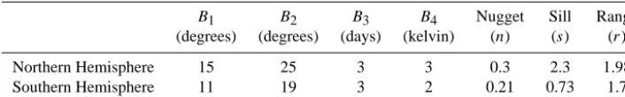
We apply Eq. (1) to TCCON data between July 2009 and April 2013 at the 16 chosen TCCON locations. For each TC-CON observation, we obtain the corresponding ACOS a pri-ori information using the colocation neighborhood region de-fined in Wunch et al. (2011b); see Sect. 4 for more detail. Fig-ure 2 displays a plot of the relationship between the original TCCON retrievals versus the averaging-kernel-corrected TC-CON data. In effect, the averaging kernel correction tends to pull TCCON observations closer to the ACOS a prioriXCO2;

TCCON values that are higher than the ACOS a priori value tend to be pulled downwards, while TCCON values lower than the ACOS a prioriXCO2tend to be pulled upwards. The

Having done averaging kernel correction to put the TC-CON and ACOS retrievals on the same footing, in the next section we describe our methodology for optimally colocat-ing ACOS-GOSAT observations to any TCCON location. The colocated values will then be compared to averaging-kernel-corrected TCCON data in Sect. 4.

3 Geostatistical colocation

Our colocation methodology exists within a geostatistical framework, which is a part of the broader area of spatial statistics. Here, we briefly review that framework, give some necessary notation, and present basic derivations for estima-tion in a spatial context.

Let{Y (s):s∈D}be a hidden, real-valued spatial process on a multidimensional domain. In the application of ACOS-GOSAT and TCCON, we lets=(slat, slon, st, sT)0be a

four-dimensional vector, specifying the latitude in degrees, longi-tude in degrees, time in fractional days, and midtropospheric temperature in kelvin at 700 hPa (T700), respectively, and we assumeY (s)is theXCO2 process at locations. We assume

that the Z(s),XCO2 retrieval at locations, is a sum of the

trueXCO2process and a retrieval-error term; that is,

Z(s) = Y (s)+(s)

= t (s)+ν(s)+(s), (2)

wheret (s)is a large-scale deterministic trend term that ac-counts for seasonal and yearly trends,ν(s)is a small-scale variability term that accounts for spatial correlation, and(s) is the retrieval-error term. We also assume that we have a variogram function 2γ (si,sj), which describes the degree of

spatial dependence between any two locationssi andsjas in

the following definition:

2γ (si,sj)=var(Z(si)−Z(sj))=

E|(Z(si)−t (si))−(Z(sj)−t (sj))|2

; si,sj∈D. (3)

LetZ=(Z(s1), Z(s1), . . . , Z(sN))0be the vector of

satel-lite observations taken at N footprints around an interpo-lation points0, and letT =(t (s1), t (s1), . . . , t (s_N))0 be the correspondingN-dimensional vector of trend terms. We wish to find an estimate ofY (s0)as a linear combination of the de-trended retrievedXCO₂vectorD=(Z−T)and an unknown vector of coefficientsa0

s0; that is,

ˆ

Y (s0)=t (s0)+a0s0D, (4)

such that we minimize the expected mean-squared error minas₀E

(Y (s0)− ˆY (s0))2

, (5)

subject to the unbiasedness constrainta0

s01=1.

The solution to the constrained minimization problem in Eqs. (4) and (5) can be found using the method of Lagrange multipliers. Cressie (1993) gives the following equation for the solutionas0 that satisfies Eq. (4) and (5),

as0

λ = (6)     

γ (s1,s1) · · · γ (s1,sN) 1

..

. . .. ... ... γ (sN,s1) · · · γ (sN,sN) 1

1 · · · 1 0



   

−1

   

γ (s1,s0) .. . γ (sN,s0)

1      ,

whereλis the scalar Lagrange multiplier andas0is the vector

of kriging coefficient.

An attractive property of the geostatistical approach is that the semivariogram function can be used to calculate the pected estimation error at the interpolation location. The ex-pression for the interpolation error is as follows:

ˆ

σ (s)= a0_s

0 λ     

γ (s1,s0) .. . γ (sN,s0)

1      . (7)

Estimating the fully general semivariogram model γ (sN,s0)is a difficult problem that is prone to robustness issues when the data are sparse. To make the problem more tractable, we assume that the variogram structure of Z is isotropic under certain distance metrics. In other words, we assume that the semivariogram capturing the spatial depen-dence between any two locationsγ (s_i,s_j)is only dependent on its “distance” as in the following equation:

γ (si,sj)=γ (|si−sj|B), (8)

where| · |_Bis a modified Euclidean distance given by

|si−sj|B= (9)

s _(s

i,lat−sj,lat)2

B1

+(si,lon−sj,lon)

2

B2

+(si,t−sj,t)

2

B3

+(si,T−sj,T)

2

B4

=

q

(si−sj)0B(si−sj), (10)

and B is a diagonal 4×4 matrix whose diagonal elements (1/B1,1/B2,1/B3,1/B4) represent the scaling parameters along each of the coordinate directions: latitude, longitude, time, andT700.

3.1 Application to ACOS-GOSAT and TCCON data

For our application, we will assume certain parametric forms for the trendt (·)and the semivariogram functionγ (·,·)and estimate the corresponding parameters along with B from the retrieved data.

Unfortunately, ACOS-GOSAT data are quite sparse once we pass the radiances through a cloud filter, retrieval selec-tion criteria, and post-retrieval data quality filters. The rel-ative global sparseness of the ACOS-GOSAT data makes it difficult to obtain robust estimates of the scaling matrix B and the semivariogram functionγ (·,·). We address this prob-lem by using CarbonTracker model XCO₂ data to estimate these spatial–temporal dependence parameters. Our assump-tion here is that CarbonTracker and ACOS-GOSAT share the same medium- to large-scale spatiotemporal dependence structure for XCO₂. For instance, the dynamics in Carbon-Tracker should reasonably approximate synoptic- and large-scale dependence in moderately homogeneous areas such as the Southern Hemisphere. Note that this assumption is not as restrictive as the assumption that CarbonTracker and ACOS-GOSAT have the same expected value ofXCO2 at every

lo-cation.

CarbonTracker is a CO2 assimilation system developed by the National Oceanic and Atmospheric Administration (NOAA) to keep track of the global CO2 emissions and uptake. The model combines surface air samples collected around the globe and from tall towers and small aircraft in North America with an atmospheric transport model coupled with a Kalman filter to produce estimates of atmospheric CO2 mole fractions on a global grid (Peters et al., 2007). The modelXCO₂ data are regularly gridded at 1◦×1◦daily resolution, making it particularly convenient for use in spa-tial parameter estimation. We use 2 years’ worth of Carbon-Tracker data (CT2001_oi) between January 2009 and De-cember 2010 in estimating the trendt (·), the scaling matrix B and the semivariogram functionγ (·,·).

3.2 Trend terms

The trend termt (·)is a deterministic term that accounts for the annual increase in XCO2 as well as the seasonal

vari-ations. This deterministic trend needs to be modeled, esti-mated, and removed from the data in Eq. (2) before we can apply the geostatistical colocation on the remaining stochas-tic terms in Eq. (4). We assume that the trend term in Eq. (4) can be modeled as a mixture of a linear constant trend and a seasonal sinusoidal trend,

t (s)=c0(s)+c1(s)st+a(s)·sin(2π st+θ (s)), (11)

wherec0(s)is they intercept andc1(s)the slope of the lin-ear portion,a(s)is the amplitude of the seasonal sinusoidal variability, andθ (s)is the sinusoidal phase shift. The period for seasonal variability is assumed to be 1 year, andst is the

time as a year fraction starting at 0 for 1 January 2009.

380 385 390 395

380

385

390

395

Original vs AK-Corrected TCCON

Original TCCON

AK-C

orre

ct

ed

T

C

C

O

N

Figure 2. Matched TCCON original daily median observations vs. averaging-kernel-corrected TCCON values. The red line is the lin-ear regression line, while the blue is the 1 : 1 line.

We make a simplifying assumption that the annual and seasonal trends are constant over the hemispheres. We aggregate daily CarbonTracker XCO₂ values over both the Northern and Southern Hemisphere for the entire 2-year period, and we compute the trend coefficients

{c0(s), c1(s), a(s), θ (s)} using variable transformation and linear regression (Artis et al., 2007). The resulting coeffi-cients are displayed in Table 1.

Table 1 indicate that the Northern Hemisphere tends to have higherXCO₂ than the Southern Hemisphere. The inter-cept term is higher for the Northern Hemisphere, indicating that the baseXCO2there is higher, and the slope is marginally

higher as well (2.61 vs. 2.49 ppm year−1), indicating that the Northern Hemisphere has a higher rate ofXCO2increase. The

main differences between the hemispheres are the amplitudes and the phase shifts of the seasonal terms. CarbonTracker in-dicates that the Northern Hemisphere has a seasonal variabil-ity with an amplitude of 3.2 ppm, while the Southern Hemi-sphere has a much lower seasonal amplitude of 0.31 ppm. The phase shifts (0.16 vs. 4.10) differ by about half a year, which is consistent with the opposite seasons in the hemi-spheres.

2009.0 2009.5 2010.0 2010.5 2011.0

384

386

388

390

392

394

396

Northern Hemisphere Mean XCO2

Year

Me

an

C

O

2

Trend Fit CarbonTracker Data

2009.0 2009.5 2010.0 2010.5 2011.0

384

386

388

390

392

394

396

Southern Hemisphere Mean XCO2

Year

Me

an

C

O

2

Trend Fit

CarbonTracker Data

Figure 3. Plots of averaged CarbonTracker trend versus sinusoidal trend fit for the Northern Hemisphere (left) and Southern Hemisphere (right).

3.3 Parameter estimation

Having modeled and estimated the trend term t (·), we now estimate the scaling matrix B and the semivariogram func-tion γ (·,·). We model the semivariogram function with the spherical semivariogram, which has the form

γ (si,sj)≡γ (h)=

(s−n)

_3h

2r − h3 2r3

1(0,r)(h)+1[r,∞)(h)

+n, (12) whereh= |si−sj|B is the modified Euclidean distance

be-tween si andsj; 1S(h) is 1 ifh∈S, and 0 otherwise, the

term nis the nugget, which denotes the height of the semi-variogram at the origin where h=0; the term s is called the sill, which is the limit of the semivariogram ash→ ∞; and r is the range, which is the distance at which the dif-ference between the semivariogram and the sill is negligible (see Cressie, 1993, for more detail).

Given the scaling matrix B, we can estimate the semivar-iogram parameters {n, s, r}by constructing the robust em-pirical semivariogram estimator discussed in Cressie (1980) and Cressie (1993, Sect. 2.4) from the CarbonTracker data as follows. Forh >0, define

2γ (h)¯ ≡

n

1 |N (h)|

P

N (h)|D(sm)−D(sn)|

1 2

o4

0.457+_|0.494

N (h)|

, (13)

whereD(s)is the detrended CarbonTracker value at location

s, andN (h)is the set of observation pairs that are separated by a distance ofh,

N (h) ≡ {(sn,sm): |sn−sm|B∗=h; m, n=1, . . . , N}. In practice, the setN (h)is defined using a small tolerance interval around h, since it may not be possible to find pairs of locations that are exactly distancehapart (Cressie, 1993, p. 70). The term|N (h)| denotes the number of unique ele-ments inN (h).

We assume that the scaling matrix B and the semivari-ogram functionγ (·,·)are constant with respect to each hemi-sphere and with respect to time. To estimate the scaling ma-trix B, we construct empirical semivariograms using data pairs that only approximately differ in one of the four co-ordinates. This effectively sets three of the four terms on the right-hand side of Eq. (9) to zero (or very close to zero), al-lowing us to estimate the single remaining scaling parameter, Bi. For instance, to estimate the scaling parameter along the

longitudinal direction, we search through the CarbonTracker data for the corresponding hemisphere to obtain pairs of ob-servations that share the same date, latitude, andT700 but different longitudes. We then calculate the robust semivar-iogram estimator in Eq. (13), compute the corresponding semivariogram fit to the spherical model in Eq. (12), and set the scaling parameterBi equal to the resulting ranger.

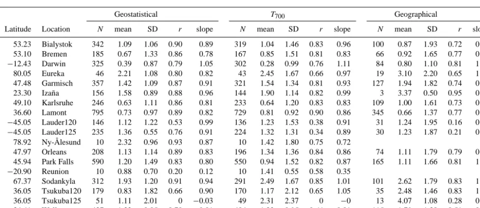
Table 2 contains the list of scaling parameters for the Northern Hemisphere and the Southern Hemisphere. In gen-eral, the scaling parameters agree fairly well with the coinci-dence windows given in Wunch et al. (2011b)’sT700 method-ology. For the Northern Hemisphere, the scaling parame-ters for latitude, longitude, time, andT700 are 15.1, 24.5, 3, and 3.1, respectively; the corresponding parameters for the Southern Hemisphere are 11.6, 19.3, 3, and 2.3. This indi-cates that in general the Northern Hemisphere has longer spa-tial correlation range than the Southern Hemisphere.

Having estimated the scaling parameters B, we construct a set of empirical semivariogram values using Eq. (13) for each of the hemispheres and estimate the semivariogram pa-rameters{n, s, r}using an iterative Gauss–Newton fitting al-gorithm to fit to the chosen spherical semivariogram model to the empirical semivariogram estimates (Cressie, 1985). The resulting nugget, sill, and range parameters for the Northern and Southern Hemisphere are presented in Table 2.

Table 2. Scaling coefficients and semivariogram parameters for Eq. (9).

B1 B2 B3 B4 Nugget Sill Range (degrees) (degrees) (days) (kelvin) (n) (s) (r) Northern Hemisphere 15 25 3 3 0.3 2.3 1.98 Southern Hemisphere 11 19 3 2 0.21 0.73 1.7

Hemisphere. Having estimated the parameters for B and γ (si,sj), we can compute the colocated ACOS-GOSAT

value at any TCCON location using Eqs. (4) and (6).

4 Comparison to existing methodologies

Having outlined the geostatistical colocation methodology in Sect. 3, we now assess its performance relative to existing methodologies, which include geographical colocation and Wunch et al. (2011a)’s T700 colocation. Our primary stan-dard for comparison is the root-mean-squared error (RMSE) between TCCON and colocated ACOS-GOSAT data. This RMSE is the sum of the variability from various sources such as the underlying atmospheric variability, GOSAT and TC-CON measurement errors, relative bias, and interpolation er-ror resulting from colocation. In this experiment, we manip-ulate the magnitude of the interpolation error by varying the method of colocation. The resulting changes in total RMSE should be indicative of the corresponding changes in interpo-lation error.

Geographical colocation methodology is perhaps the most popular colocation methodology due to its simplicity and straightforwardness. Examples of geographical coincident criteria include selecting all same-day satellite observations falling within ±5◦ of a location of interest (Inoue et al., 2013), selecting data falling within±30 min from about 0.5 to 1.5◦ rectangles centered at each validation site (Morino et al., 2011), selecting data within 5◦ and±2 h (Butz et al., 2011; Cogan et al., 2012), selecting observations within a 10◦×10◦ lat–long box (Reuter et al., 2013), and select-ing weekly data that fall within a 5◦ radius of a validation site (Oshchepkov et al., 2012). For the performance com-parison in this section, we define a geographical colocation methodology by averaging all same-day satellite observa-tions falling within 500 km of a location of interest. This colocation methodology is based on the one used in Inoue et al. (2013), with the exception that we replace the lat–long circle with a great-distance circle to avoid warping near the poles.

Wunch et al. (2011b) refined the geographical method by adding midtropospheric temperature at 700 hPa as an extra threshold to take advantage of the correlation betweenXCO2

and midtropospheric temperature (Keppel-Aleks et al., 2011, 2012). Their colocation methodology locates and averages all ACOS-GOSAT observations falling within ±30◦ longi-tude, ±10◦ latitude,±5 days, and±2 kelvin inT700. The

longitudinal constraint is reduced to±10◦ for the Tsukuba TCCON site to avoid inordinate influence from ACOS-GOSAT retrievals over China. In this section, we assess the performance of Wunch et al. (2011b)’s colocation cri-terion and the geographical method relative to geostatistical colocation methodology between the period July 2009 and April 2013.

4.1 Comparison between ACOS-GOSAT and TCCON data

For the performance assessment, we use all available TC-CON data from 16 locations (4 in the Southern Hemisphere, 12 in the Northern Hemisphere; see Fig. 1) between the period July 2009 and April 2013. Since the three coloca-tion methodologies compute averages over large temporal spans, applying the three methodologies to individual same-station TCCON observations (which may be spaced seconds or minutes apart from one another) would result in a scenario where many temporally proximal TCCON observations are matched to the same ACOS-GOSAT colocated value. We avoid this problem by taking the daily median of TCCON XCO₂ values and using them as the standard against which we assess the outputs of the colocation methodologies.

Having taken the daily median of the TCCONXCO2

val-ues, we scan the entire TCCON data set and locate corre-sponding matches using the colocation methodologies. At every TCCON location and every day for which we have a daily median TCCONXCO2 value, we gather the

corre-sponding ACOS-GOSAT values falling within the respec-tive coincidence regions and then compute the colocated value for each of the three methodologies. Some TCCON locations may not have a corresponding colocated ACOS-GOSAT value for particular days due to the fact that they do not have any GOSAT values within their coincidence neigh-borhood. The neighborhood regions are constructed sepa-rately for each TCCON location, and thus some ACOS-GOSAT sounding may be used more than once in comput-ing the colocated values for several temporally or spatially proximal TCCON daily median values.

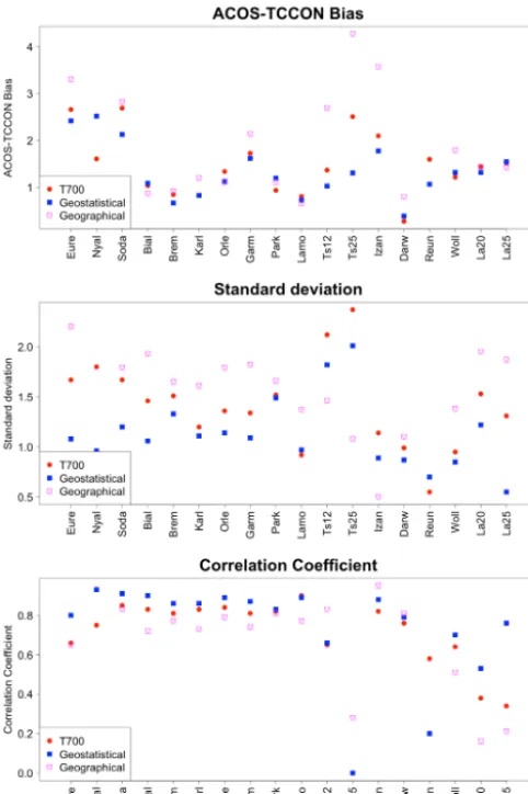
Figure 4. TCCON daily median (black) vs.T700(red), geostatistical (blue), and geographical (green) colocation values. Time in days is displayed on thexaxis, whileXCO2concentration in ppm is displayed on theyaxis. Reunion and Tsukuba125 data sets are omitted due to

the low number of observations.

a lot more colocated values due the fact that they use data from a large spatiotemporal neighborhood surrounding a TC-CON site. From Fig. 4, all colocation methodologies indi-cate that ACOS-GOSAT XCO2 tends to be larger than

TC-CONXCO₂ and the magnitude of this bias is between 1 and 1.5 ppm. Northern TCCON sites such as Eureka and Ny-Ålesund do not have nearby ACOS-GOSAT H-gain good-quality retrievals during the winter due to ice and snow is-sues.

Table 4 displays five ACOS-GOSAT/TCCON summary statistics: number of matched days (N), mean bias, stan-dard deviation, correlation coefficient (r), and slope. Geo-statistical and T700 methodologies have wider coincidence

criteria than our chosen geographical methodology, and con-sequently have more daily matched ACOS-GOSAT/TCCON pairs. To better examine the patterns in Table 4, we display the main statistics (bias, standard deviation, and correlation coefficient) in graphical form in Fig. 5, with the TCCON sta-tions listed in order of decreasing latitude.

Table 3. Overall mean-squared error for the three colocation methodologies before and after averaging kernel (AK) correction on TCCON. Units are ppm.

T700 Geographical Geostatistical Before AK correction 1.57 1.88 1.43 After AK correction 1.45 1.60 1.22

Table 4. Overall summary statistics for the three colocation methodologies. Statistics include number of matched days (N), mean bias, standard deviation (SD), correlation coefficient (r), and slope.

Geostatistical T₇₀₀ Geographical

Latitude Location N mean SD r slope N mean SD r slope N mean SD r slope

53.23 Bialystok 342 1.09 1.06 0.90 0.89 319 1.04 1.46 0.83 0.96 100 0.87 1.93 0.72 0.95 53.10 Bremen 185 0.67 1.33 0.86 0.78 167 0.85 1.51 0.81 0.83 66 0.92 1.65 0.77 0.86 −12.43 Darwin 325 0.39 0.87 0.79 1.05 302 0.28 0.99 0.76 1.11 84 0.80 1.10 0.81 1.22 80.05 Eureka 46 2.21 1.08 0.80 0.82 43 2.45 1.67 0.66 0.97 19 3.10 2.20 0.65 1.19 47.48 Garmisch 357 1.42 1.09 0.87 0.91 321 1.54 1.34 0.81 0.93 127 1.94 1.82 0.74 0.95 23.30 Izaña 156 1.58 0.89 0.88 0.96 144 1.90 1.14 0.82 0.99 3 3.37 0.50 0.95 0.99 49.10 Karlsruhe 246 0.63 1.11 0.86 0.81 233 0.64 1.20 0.83 0.83 109 1.00 1.61 0.73 0.83 36.60 Lamont 795 0.73 0.97 0.89 0.82 729 0.81 0.92 0.90 0.86 345 0.66 1.37 0.77 0.81 −45.05 Lauder120 146 1.12 1.22 0.53 0.99 136 1.23 1.53 0.38 0.91 31 1.24 1.95 0.16 0.62 −45.05 Lauder125 235 1.36 0.55 0.76 0.91 224 1.32 1.31 0.34 0.89 30 1.23 1.87 0.21 0.92

78.92 Ny-Ålesund 10 2.32 0.96 0.93 0.87 10 1.42 1.80 0.75 0.72

47.97 Orleans 208 1.13 1.14 0.89 0.83 196 1.34 1.36 0.84 0.86 74 1.11 1.79 0.79 0.87 45.94 Park Falls 590 1.20 1.49 0.83 0.80 550 0.94 1.52 0.82 0.87 165 1.11 1.66 0.81 1.06 −20.90 Reunion 10 0.88 0.70 0.20 0.12 10 1.41 0.55 0.58 0.35

67.37 Sodankyla 312 1.93 1.20 0.91 0.94 291 2.49 1.67 0.85 1.01 101 2.62 1.79 0.83 1.09 36.05 Tsukuba120 179 0.83 1.82 0.66 0.90 170 1.17 2.12 0.65 1.05 35 2.48 1.46 0.83 1.14 36.05 Tsukuba125 51 1.11 2.01 0 −0.03 49 2.31 2.37 0 −0 13 4.07 1.08 0.28 0.45 −34.41 Wollongong 437 1.32 0.85 0.70 0.81 404 1.22 0.95 0.64 0.81 115 1.79 1.38 0.51 0.88

pronounced variability in the estimates of mean bias at the TCCON sites. This is likely due to the fact that the geo-graphical method has a much smaller neighborhood region, and thus does not yield enough colocated matches relative to TCCON to produce a robust bias estimate. All three method-ologies tend to have high bias estimates for the three north-ernmost TCCON sites: Sodankyla, Eureka, and Ny-Ålesund. This is likely because soundings acquired over these snowy and icy surfaces have low reflectivity in the 1.61 and 2.06 µm bands; consequently scattering by thin clouds and aerosols can constitute a larger fraction of the total signal and in-troduce larger uncertainties in the optical path length (Crisp et al., 2012).

The clear delineating metric between the three method-ologies is the RMSE (also known as standard deviation), which we display in the middle panel of Fig. 5 on a station-by-station basis. The three methodologies are roughly sep-arated into clusters: the geographical method has on aver-age the highest RMSE,T700ranks in the middle, and geosta-tistical colocation has the lowest RMSE. One might expect the geographical method to have the lowest RMSE since it only accepts ACOS-GOSAT values within a fairly narrow spatiotemporal neighborhood (500 km same-day window). However, this is not the case since the RMSE is a function of both the spatial dependence structure and the retrieval error

characteristics. Since the GOSAT measurements tend to have relatively large single-sounding uncertainties, the T700 and the geostatistical colocation methods are able to take advan-tage of the large number of observations within the coinci-dent neighborhood to reduce the variability through the law of large numbers.

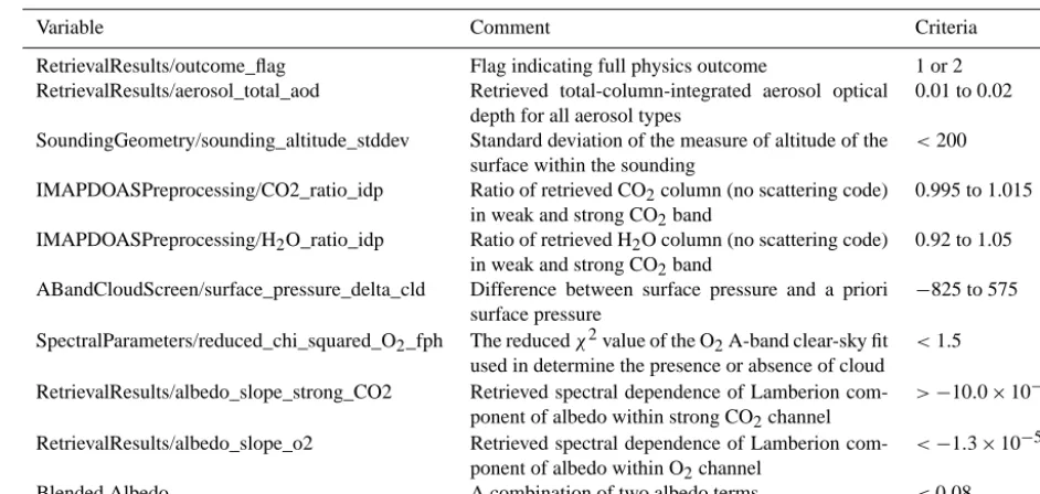
Table 5. Advanced screening criteria for ACOS v3.3 L2 H-gain data (Osterman et al., 2013, Sect. 2.5.2).

Variable Comment Criteria

RetrievalResults/outcome_flag Flag indicating full physics outcome 1 or 2 RetrievalResults/aerosol_total_aod Retrieved total-column-integrated aerosol optical

depth for all aerosol types

0.01 to 0.02

SoundingGeometry/sounding_altitude_stddev Standard deviation of the measure of altitude of the surface within the sounding

<200

IMAPDOASPreprocessing/CO2_ratio_idp Ratio of retrieved CO2column (no scattering code) in weak and strong CO2band

0.995 to 1.015

IMAPDOASPreprocessing/H2O_ratio_idp Ratio of retrieved H2O column (no scattering code) in weak and strong CO2band

0.92 to 1.05

ABandCloudScreen/surface_pressure_delta_cld Difference between surface pressure and a priori surface pressure

−825 to 575

SpectralParameters/reduced_chi_squared_O₂_fph The reducedχ2value of the O₂A-band clear-sky fit used in determine the presence or absence of cloud

<1.5

RetrievalResults/albedo_slope_strong_CO2 Retrieved spectral dependence of Lamberion com-ponent of albedo within strong CO2channel

>−10.0×10−5

RetrievalResults/albedo_slope_o2 Retrieved spectral dependence of Lamberion com-ponent of albedo within O2channel

<−1.3×10−5

Blended Albedo A combination of two albedo terms <0.08

derived, compared to the other colocation methodologies in this section, is more reflective and representative of the true underlying dependence structure.

Another way to assess the fit between ACOS-GOSAT and TCCON values is through examining the correlation coeffi-cient. Since the satellite and station instruments both observe total-columnXCO₂, we expect the two to follow a linear rela-tionship with a slope of 1 and ayintercept equal to the mean bias. The correlation coefficient is a good tool to examine the strength and direction of the linear relationship between the ACOS-GOSAT and TCCON values, and we show the corre-lation estimates at each of the TCCON sites in the bottom panel of Fig. 5.

In our particular application, correlation values closer to 1 indicate stronger linear dependence. In this respect, geosta-tistical colocation performs marginally better thanT700 cation, and they both perform better than geographical colo-cation. The correlation estimates mostly cluster within the range of 0.75 to 0.99, with the exception being TCCON sta-tions in the Southern Hemisphere. This likely results from the fact that the Northern Hemisphere and the Southern Hemi-sphere have a different seasonal and synoptic variability ra-tio. In general, the ACOS-GOSAT retrievals do quite well in capturing the overall seasonal trends in both hemispheres. However, in the Northern Hemisphere, the seasonal variabil-ity amplitude is larger than the synoptic variabilvariabil-ity, and con-sequently the correlation coefficient between ACOS-GOSAT and TCCON is larger. In the Southern Hemisphere, the sea-sonal variability amplitude is much smaller at 0.3 ppm, thus lowering the correlation coefficient.

The comparisons in this section indicate that, in general, geographical colocation has low matching yield and poor ac-curacy performance. This is likely because the geographi-cal colocation used (same-day 500 km circle) lacks the large coincident neighborhood to reduce the individual retrieval variability through averaging. Wunch et al.’s (2011) T700 and geostatistical colocation both take advantage of a larger colocation neighborhood to produce more accurate ACOS-GOSAT colocated values.

While these methodologies produce roughly the same bias estimates, geostatistical colocation produces distinctly lower RMSE. This improvement likely comes from the fact that while the existing colocation methodologies tend to give equal weights to all satellite observations falling within the coincident window, our methodology gives different weights to the coincident satellite observations based on the distance metric defined in Eq. (10).XCO₂ in general tends to be a smoothly varying field and it can be reasonably assumed to follow the geographical principle that locations close to one another are more likely to be similar than locations far apart (Tobler, 1970); therefore our methodology produces better accuracy because its spatial-dependency model is more re-flective and representative of the true underlyingXCO₂ field.

5 Conclusions

Figure 5. Summary statistics for the comparison between ACOS and TCCON using three colocation methodologies (top panel: bias; middle panel: standard deviation; bottom panel: correlation coeffi-cients). TCCON stations are listed in order of decreasing latitude.

of the difference between validation and colocated data; it is important to minimize the interpolation error as much as possible in order to better assess important instrumental and operational metrics such as bias and variability relative to the validation data.

This paper examines a new colocation technique in com-paring ACOS-GOSAT and TCCON data. We model the spa-tial dependence structure as being isotropic under a modi-fied Euclidean distance metric. Our methodology is similar to previous colocation techniques (e.g., geographical,T700, model-based) in that we assume that nearby observations are more likely to be correlated than observations far apart. How-ever, whereas the existing methodologies define some neigh-borhood regions and then give all neighboring observations equal weights, our methodology weights each observation depending on the distances between the data and the inter-polation location of interest.

In Sect. 4, we show that our geostatistical colocation methodology has the lowest mean-squared error of the dif-ference between colocated ACOS-GOSAT data and TCCON data when compared with two existing colocation method-ologies. Naturally, one would expect the correlation structure in ACOS-GOSATXCO2to vary smoothly as a function of

dis-tance, and hence our method has better performance because its spatial correlation model is more approximate to the true underlying spatial structure. While we applied the methodol-ogy in Sect. 3 to ACOS-GOSAT and TCCON data, the colo-cation methodology can be readily applied to other satellite instruments and other geophysical processes where the un-derlying correlation structure can be reasonably assumed to vary smoothly as a function of distance.

In Sect. 3, we chose to use midtropospheric temperature as a covariate to improve our interpolation; it is possible to replaceT700 with another covariate such as 3-day-averaged modelXCO₂as in the model-based method. While the param-eters of the resulting correlation function would change with the replacement ofT700, the parameter estimation procedure in Sect. 3.3 would remain the same. We also note that the distance metric we derived in Eq. (10) has value beyond per-forming geostatistical colocation. It could be used as a stand-alone metric in assessing proximity (e.g., findingk-nearest neighbors, computing inverse distance weighting, construct-ing Voronoi diagrams, etc.).

In this paper we assumed that ACOS-GOSAT retrievals can be approximated and treated as zero-area points. In certain applications it may be more reasonable to assume that a satellite observation is an average of the true geo-physical process Y (·)over the area of the footprint plus a measurement-error term. The resulting process of inferring a spatial process at one resolution from data at another resolu-tion, also known as the change-of-support problem, is more complex; see Gotway and Young (2002) for a review. In gen-eral, there is no analytical solution for estimating the pa-rameters of standard variogram models from areal data (e.g., spherical, exponential, etc.); however, certain classes of spa-tial models provide for straightforward and seamless parame-ter estimation (for instance, see spatial random effects model; Cressie and Johannesson, 2008; Nguyen et al., 2012).

Acknowledgements. This research was carried out at the Jet Propulsion Laboratory, California Institute of Tech-nology, under a contract with NASA. ACOS data are ob-tained from Goddard Earth Sciences Data and Informa-tion Services Center, operated by NASA, from the website http://disc.sci.gsfc.nasa.gov/acdisc/documentation/ACOS.shtml. TCCON data were obtained from the TCCON Data Archive, operated by the California Institute of Technology, from the website at http://tccon.ipac.caltech.edu/. NCEP reanalysis data are provided by the NOAA/OAR/ESRL PSD, Boulder, Colorado, USA, from their website at http://www.cdc.noaa.gov/.

Edited by: W. R. Simpson

References

ACOS Data Access: Goddard Earth Sciences Data and Information Services Center, available at: http://disc.sci.gsfc.nasa.gov/acdisc/ documentation/ACOS.shtml, last access: June 2013.

Artis, M., Clavel, J. G., Hoffmann, M., and Nachane, D.: Harmonic Regression Models: A Comparative Review with Applications, IEW – Working Papers 333, Institute for Empirical Research in Economics – University of Zurich, 2007.

Boesch, H., Baker, D., Connor, B., Crisp, D., and Miller, C.: Global Characterization of CO₂ Column Retrievals from Shortwave-Infrared Satellite Observations of the Orbiting Car-bon Observatory-2 Mission, Remote Sensing, 3, 270–304, 2011. Bosch, H., Toon, G. C., Sen, B., Washenfelder, R. A., Wennberg, P. O., Buchwitz, M., de Beek, R., Burrows, J. P., Crisp, D., Christi, M., Connor, B. J., Natraj, V., and Yung, Y. L.: Space-based near-infrared CO2 measurements: Testing the Orbiting Carbon Observatory retrieval algorithm and vali-dation concept using SCIAMACHY observations over Park Falls, Wisconsin, J. Geophys. Res. Atmos., 111, D23302, doi:10.1029/2006JD007080, 2006.

Bovensmann, H., Burrows, J., Buchwitz, M., Frederick, J., Noel, S., Rozanov, V. V., Chance, K. V., and Geode, A. P. H.: SCIA-MACHY: Mission objectives and measurement modes, J. Atmos. Sci., 56, 127–150, 1999.

Butz, A., Guerlet, S., Jacob, D. J., Schepers, D., Galli, A., Aben, I., Frankenberg, C., Hartmann, J.-M., Tran, H., Kuze, A., Keppel-Aleks, G., Toon, G. C., Wunch, D., Wennberg, P. O., Deutscher, N. M., Griffith, D. W. T., Macatangay, R., Messerschmidt, J., Notholt, J., and Warneke, T.: Toward accurate CO2and CH4 ob-servations from GOSAT, Geophys. Res. Lett., 38, 2–7, 2011. Cogan, A. J., Boesch, H., Parker, R. J., Feng, L., Palmer, P. I.,

Blavier, J.-F. L., Deutscher, N. M., Macatangay, R., Notholt, J., Roehl, C., Warneke, T., and Wunch, D.: Atmospheric carbon dioxide retrieved from the Greenhouse gases Observing SATel-lite (GOSAT): Comparison with ground-based TCCON obser-vations and GEOS-Chem model calculations, J. Geophys. Res. Atmos., 117, D21301, doi:10.1029/2012JD018087, 2012. Connor, B. J., Boesch, H., Toon, G., Sen, B., Miller, C., and Crisp,

D.: Orbiting Carbon Observatory: Inverse method and prospec-tive error analysis, J. Geophys. Res. Atmos., 113, D05305, doi:10.1029/2006JD008336, 2008.

Cressie, N.: M-estimation in the presence of unequal scale, Statis-tica Neerlandica, 34, 19–32, 1980.

Cressie, N.: Fitting Variogram Models by Weighted Least Squares, Mathematical Geology, 17, 563–570, 1985.

Cressie, N.: Statistics for Spatial Data, revised edition, Wiley-Interscience, New York, NY, 1993.

Cressie, N. and Johannesson, G.: Fixed rank kriging for very large spatial data sets, J. Roy. Stat. Soc. Ser. B, 70, 209–226, 2008. Crisp, D., Fisher, B. M., O’Dell, C., Frankenberg, C., Basilio, R.,

Bösch, H., Brown, L. R., Castano, R., Connor, B., Deutscher, N. M., Eldering, A., Griffith, D., Gunson, M., Kuze, A., Man-drake, L., McDuffie, J., Messerschmidt, J., Miller, C. E., Morino, I., Natraj, V., Notholt, J., O’Brien, D. M., Oyafuso, F., Polonsky, I., Robinson, J., Salawitch, R., Sherlock, V., Smyth, M., Suto, H., Taylor, T. E., Thompson, D. R., Wennberg, P. O., Wunch, D., and Yung, Y. L.: The ACOS CO2retrieval algorithm – Part II: Global XCO2data characterization, Atmos. Meas. Tech., 5, 687—707, doi:10.5194/amt-5-687-2012, 2012.

Deutscher, N. M., Griffith, D. W. T., Bryant, G. W., Wennberg, P. O., Toon, G. C., Washenfelder, R. A., Keppel-Aleks, G., Wunch, D., Yavin, Y., Allen, N. T., Blavier, J.-F., Jiménez, R., Daube, B. C., Bright, A. V., Matross, D. M., Wofsy, S. C., and Park, S.: Total column CO2measurements at Darwin, Australia – site de-scription and calibration against in situ aircraft profiles, Atmos. Meas. Tech., 3, 947–958, doi:10.5194/amt-3-947-2010, 2010. Gotway, C. A. and Young, L. J.: Combining Incompatible Spatial

Data, J. Am. Stat. Assoc., 97, 632–648, 2002.

Gruber, N., Gloor, M., Fletcher, S. E. M., Dutkiewicz, S., Fol-lows, M., Doney, S. C., Gerber, M., Jacobson, A. R., Lindsay, K., Menemenlis, D., Mouchet, A., Mueller, S. A., Sarmiento, J. L., and Takahashi, T.: Oceanic sources, sinks, and transport of atmospheric CO2, Global Biogeochem. Cy., 23, GB1005, doi:10.1029/2008GB003349, 2009.

Guerlet, S., Butz, A., Schepers, D., Basu, S., Hasekamp, O. P., Kuze, A., Yokota, T., Blavier, J.-F., Deutscher, N. M., Griffith, D. W., Hase, F., Kyro, E., Morino, I., Sherlock, V., Sussmann, R., Galli, A., and Aben, I.: Impact of aerosol and thin cirrus on retrieving and validating XCO2 from GOSAT shortwave infrared measurements, J. Geophys. Res. Atmos., 118, 4887–4905, 2013. Hamazaki, T., Kaneko, Y., Kuze, A., and Kondo, K.: Fourier trans-form spectrometer for Greenhouse Gases Observing Satellite (GOSAT), in: Society of Photo-Optical Instrumentation Engi-neers (SPIE) Conference Series, edited by: Komar, G. J., Wang, J., and Kimura, T., vol. 5659 of Society of Photo-Optical Instru-mentation Engineers (SPIE) Conference Series, 73–80, 2005. Inoue, M., Morino, I., Uchino, O., Miyamoto, Y., Yoshida, Y.,

Yokota, T., Machida, T., Sawa, Y., Matsueda, H., Sweeney, C., Tans, P. P., Andrews, A. E., Biraud, S. C., Tanaka, T., Kawakami, S., and Patra, P. K.: Validation of XCO2 derived from SWIR spectra of GOSAT TANSO-FTS with aircraft measurement data, Atmos. Chem. Phys., 13, 9771–9788, doi:10.5194/acp-13-9771-2013, 2013.

Kalnay, E., Kanamitsu, M., Kistler, R., Collins, W., Deaven, D., Gandin, L., Iredell, M., Saha, S., White, G., Woollen, J., Zhu, Y., Leetmaa, A., and Reynolds, R.: The NCEP/NCAR 40-Year Re-analysis Project, Bull. Am. Meteorol. Soc., 77, 437–471, 1996. Keppel-Aleks, G., Wennberg, P. O., and Schneider, T.: Sources of

variations in total column carbon dioxide, Atmos. Chem. Phys., 11, 3581–3593, doi:10.5194/acp-11-3581-2011, 2011.

Con-nor, B., Davis, K. J., Desai, A. R., Messerschmidt, J., Notholt, J., Roehl, C. M., Sherlock, V., Stephens, B. B., Vay, S. A., and Wofsy, S. C.: The imprint of surface fluxes and transport on vari-ations in total column carbon dioxide, Biogeosciences, 9, 875– 891, doi:10.5194/bg-9-875-2012, 2012.

Messerschmidt, J., Geibel, M. C., Blumenstock, T., Chen, H., Deutscher, N. M., Engel, A., Feist, D. G., Gerbig, C., Gisi, M., Hase, F., Katrynski, K., Kolle, O., Lavriˇc, J. V., Notholt, J., Palm, M., Ramonet, M., Rettinger, M., Schmidt, M., Suss-mann, R., Toon, G. C., Truong, F., Warneke, T., Wennberg, P. O., Wunch, D., and Xueref-Remy, I.: Calibration of TCCON column-averaged CO2: the first aircraft campaign over Euro-pean TCCON sites, Atmos. Chem. Phys., 11, 10765–10777, doi:10.5194/acp-11-10765-2011, 2011.

Morino, I., Uchino, O., Inoue, M., Yoshida, Y., Yokota, T., Wennberg, P. O., Toon, G. C., Wunch, D., Roehl, C. M., Notholt, J., Warneke, T., Messerschmidt, J., Griffith, D. W. T., Deutscher, N. M., Sherlock, V., Connor, B., Robinson, J., Sussmann, R., and Rettinger, M.: Preliminary validation of column-averaged vol-ume mixing ratios of carbon dioxide and methane retrieved from GOSAT short-wavelength infrared spectra, Atmos. Meas. Tech., 4, 1061–1076, doi:10.5194/amt-4-1061-2011, 2011.

Nguyen, H., Cressie, N., and Braverman, A.: Spatial statistical data fusion for remote sensing applications, J. Am. Stat. Assoc., 107, 1004–1018, 2012.

O’Dell, C. W., Connor, B., Bösch, H., O’Brien, D., Frankenberg, C., Castano, R., Christi, M., Eldering, D., Fisher, B., Gunson, M., McDuffie, J., Miller, C. E., Natraj, V., Oyafuso, F., Polonsky, I., Smyth, M., Taylor, T., Toon, G. C., Wennberg, P. O., and Wunch, D.: The ACOS CO2retrieval algorithm – Part 1: Description and validation against synthetic observations, Atmos. Meas. Tech., 5, 99–121, doi:10.5194/amt-5-99-2012, 2012.

Oshchepkov, S., Bril, A., Yokota, T., Morino, I., Yoshida, Y., Mat-sunaga, T., Belikov, D., Wunch, D., Wennberg, P. O., Toon, G. C., O’Dell, C. W., Butz, A., Guerlet, S., Cogan, A., Boesch, H., Eguchi, N., Deutscher, N. M., Griffith, D., Macatangay, R., Notholt, J., Sussmann, R., Rettinger, M., Sherlock, V., Robinson, J., Kyrö, E., Heikkinen, P., Feist, D. G., Nagahama, T., Kady-grov, N., Maksyutov, S., Uchino, O., and Watanabe, H.: Effects of atmospheric light scattering on spectroscopic observations of greenhouse gases from space: Validation of PPDF-based CO2 re-trievals from GOSAT, J. Geophys. Res., 117, 1–18, 2012. Osterman, G., Eldering, A., Avis, C., O’Dell, C., Martinez, E.,

Frankenberg, C., Fisher, B., and Wunch, D.: ACOS Level 2 Stan-dard Product Data User’s Guide v3.3, Revision Date: Revision G, 13 June 2013, available at: http://oco.jpl.nasa.gov/files/oco/ ACOS_v3.3_DataUsersGuide.pdf, 2013.

Peters, W., Jacobson, A. R., Sweeney, C., Andrews, A. E., Con-way, T. J., Masarie, K., Miller, J. B., Bruhwiler, L. M. P., Pétron, G., Hirsch, A. I., Worthy, D. E. J., van der Werf, G. R., Ran-derson, J. T., Wennberg, P. O., Krol, M. C., and Tans, P. P.: An atmospheric perspective on North American carbon diox-ide exchange: CarbonTracker, Proc. Natl. Aca. Sci., 104, 18925– 18930, 2007.

Reuter, M., Bösch, H., Bovensmann, H., Bril, A., Buchwitz, M., Butz, A., Burrows, J. P., O’Dell, C. W., Guerlet, S., Hasekamp, O., Heymann, J., Kikuchi, N., Oshchepkov, S., Parker, R., Pfeifer, S., Schneising, O., Yokota, T., and Yoshida, Y.: A joint effort to deliver satellite retrieved atmospheric CO2concentrations for

surface flux inversions: the ensemble median algorithm EMMA, Atmos. Chem. Phys., 13, 1771–1780, doi:10.5194/acp-13-1771-2013, 2013.

Rodgers, C. D.: Inverse methods for atmospheric sounding: theory and practice, vol. 2 of Series on atmospheric, oceanic and plane-tary physics, World Scientific, River Edge, N.J., 2000.

Rodgers, C. D. and Connor, B. J.: Intercomparison of remote sounding instruments, J. Geophys. Res. Atmos., 108, 4116, doi:10.1029/2002JD002299, 2003.

TCCON Data Access: TCCON Data Archive, available at: http://tccon.ipac.caltech.edu/, recommended bias corrections: https://tccon-wiki.caltech.edu/Network_Policy/Data_Use_ Policy/Data_Description#Laser_Sampling_Errors, last access: June 2013.

Tobler, W.: A computer movie simulating urban growth in the De-troit region, Economic Geography, 46, 234–240, 1970.

Washenfelder, R. A., Toon, G. C., Blavier, J.-F., Yang, Z., Allen, N. T., Wennberg, P. O., Vay, S. A., Matross, D. M., and Daube, B. C.: Carbon dioxide column abundances at the Wis-consin Tall Tower site, J. Geophys. Res. Atmos., 111, D22305, doi:10.1029/2006JD007154, 2006.

Wunch, D., Toon, G. C., Wennberg, P. O., Wofsy, S. C., Stephens, B. B., Fischer, M. L., Uchino, O., Abshire, J. B., Bernath, P., Bi-raud, S. C., Blavier, J.-F. L., Boone, C., Bowman, K. P., Browell, E. V., Campos, T., Connor, B. J., Daube, B. C., Deutscher, N. M., Diao, M., Elkins, J. W., Gerbig, C., Gottlieb, E., Griffith, D. W. T., Hurst, D. F., Jiménez, R., Keppel-Aleks, G., Kort, E. A., Macatangay, R., Machida, T., Matsueda, H., Moore, F., Morino, I., Park, S., Robinson, J., Roehl, C. M., Sawa, Y., Sherlock, V., Sweeney, C., Tanaka, T., and Zondlo, M. A.: Calibration of the Total Carbon Column Observing Network using aircraft profile data, Atmos. Meas. Tech., 3, 1351—1362, doi:10.5194/amt-3-1351-2010, 2010.

Wunch, D., Toon, G., Blavier, J., Washenfelder, R., Notholt, J., Con-nor, B., Griffith, D., Sherlock, V., and Wennberg, P.: The Total Carbon Column Observing Network, Philos. Trans. Roy. Soc. A, 369, 2087–2112, 2011a.

Wunch, D., Wennberg, P. O., Toon, G. C., Connor, B. J., Fisher, B., Osterman, G. B., Frankenberg, C., Mandrake, L., O’Dell, C., Ahonen, P., Biraud, S. C., Castano, R., Cressie, N., Crisp, D., Deutscher, N. M., Eldering, A., Fisher, M. L., Griffith, D. W. T., Gunson, M., Heikkinen, P., Keppel-Aleks, G., Kyrö, E., Lindenmaier, R., Macatangay, R., Mendonca, J., Messerschmidt, J., Miller, C. E., Morino, I., Notholt, J., Oyafuso, F. A., Ret-tinger, M., Robinson, J., Roehl, C. M., Salawitch, R. J., Sher-lock, V., Strong, K., Sussmann, R., Tanaka, T., Thompson, D. R., Uchino, O., Warneke, T., and Wofsy, S. C.: A method for eval-uating bias in global measurements of CO2total columns from space, Atmos. Chem. Phys., 11, 12317–12337, doi:10.5194/acp-11-12317-2011, 2011b.

Yokota, T., Oguma, H., I., M., and Inoue, G.: A nadir looking SWIR FTS to monitor CO2 column density for Japanese GOSAT project, Proc. Twenty-fourth Int. Sympo. on Space Technol. and Sci. (Selected Papers), 887–889, 2004.