Solid Earth, 7, 1125–1139, 2016 www.solid-earth.net/7/1125/2016/ doi:10.5194/se-7-1125-2016
© Author(s) 2016. CC Attribution 3.0 License.
Phase segmentation of X-ray computer tomography rock images
using machine learning techniques: an accuracy
and performance study
Swarup Chauhan1, Wolfram Rühaak1,2, Hauke Anbergen3, Alen Kabdenov3, Marcus Freise3, Thorsten Wille3, and Ingo Sass1,2
1Department of Geothermal Science and Technology, Institute of Applied Geosciences, Technische Universität Darmstadt, Darmstadt, Germany
2Darmstadt Graduate School of Excellence Energy Science and Engineering, Technische Universität Darmstadt, Darmstadt, Germany
3APS Antriebs-, Prüf- und Steuertechnik GmbH, Göttingen, Rosdorf, Germany
Correspondence to:Wolfram Rühaak ([email protected], [email protected]) Received: 29 February 2016 – Published in Solid Earth Discuss.: 1 April 2016
Revised: 14 June 2016 – Accepted: 24 June 2016 – Published: 19 July 2016
Abstract. Performance and accuracy of machine learning techniques to segment rock grains, matrix and pore voxels from a 3-D volume of X-ray tomographic (XCT) grayscale rock images was evaluated. The segmentation and classifi-cation capability of unsupervised (k-means, fuzzyc-means, self-organized maps), supervised (artificial neural networks, least-squares support vector machines) and ensemble classi-fiers (bragging and boosting) were tested using XCT images of andesite volcanic rock, Berea sandstone, Rotliegend sand-stone and a synthetic sample. The averaged porosity obtained for andesite (15.8±2.5 %), Berea sandstone (16.3±2.6 %), Rotliegend sandstone (13.4±7.4 %) and the synthetic sam-ple (48.3±13.3 %) is in very good agreement with the re-spective laboratory measurement data and varies by a factor of 0.2. The k-means algorithm is the fastest of all machine learning algorithms, whereas a least-squares support vector machine is the most computationally expensive. Metrics en-tropy, purity, mean square root error, receiver operational characteristic curve and 10 K-fold cross-validation were used to determine the accuracy of unsupervised, supervised and ensemble classifier techniques. In general, the accuracy was found to be largely affected by the feature vector selection scheme. As it is always a trade-off between performance and accuracy, it is difficult to isolate one particular machine learn-ing algorithm which is best suited for the complex phase seg-mentation problem. Therefore, our investigation provides
pa-rameters that can help in selecting the appropriate machine learning techniques for phase segmentation.
1 Introduction
Micro X-ray computer tomography (XCT) images of a rock sample help in classification of pore space and assist in mod-eling of pore-network geometries. Pore-network geometries give an insight into the evolution of permeability and porosity of a rock sample. Image segmentation is the first step toward pore-network modeling. While developing this pore-network model discrimination between porous space and throat has to be resolved to the best possible extent. Currently this dis-crimination is still subjective (Piller, et al., 2009 and De Boever et al., 2012). A well-segmented 2-D or 3-D image of porous geometry provides a good foundation to obtain ef-fective permeability and porosity trends.
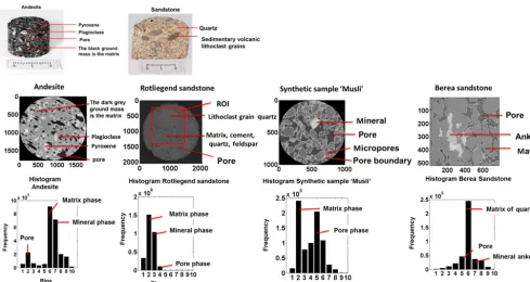
Figure 1.The top panel shows the andesite and Rotliegend sandstone rocks used for XCT measurements. Middle panel shows the raw images of andesite (16 bit), Rotliegend sandstone (16 bit), synthetic sample (16 bit) and Berea sandstone (16 bit). Mineral composition of andesite and Rotliegend sandstone was determined from thin sections using a polarized microscope. Bottom panel shows histogram plot of the respective samples. Mineral composition of Berea sandstone is based on Madonna et al. (2012) and Andrä et al. (2013).
the density of the specimen. X-ray micro computed tomog-raphy involves collecting a tomogram using high-energy X-rays to achieve very high voxel resolution.
Segmentation is the partitioning of a tomogram (grayscale image) into disjoint regions that are homogeneous with re-spect to some characteristic. Porous materials like sedimen-tary and volcanic rocks contain areas of void, called the pore space, as well as a number of distinct mineral components, each with a comparatively uniform density. These different components are referred to as phases. Segmentation of a porous rock means deciding to which phase each voxel be-longs. Tomographic images of such materials consist of a cubic array of reconstructed linear X-ray attenuation coef-ficient values each corresponding to a voxel of the sample. Ideally, one would wish to have a multi-modal distribution giving unambiguous phase separation of the pore and various mineral phase peaks. For flow properties, in particular, one would like to obtain a clear distribution separating the pore phase from mineral phase peaks. Unfortunately, the presence of low-density pore inclusions (e.g., microporosity, clays) be-low the image resolution can lead to a spread in the be- low-density signal making it difficult to unambiguously differen-tiate the pore from the microporous and solid mineral. As a consequence, significant features can be lost, and macro-scopic properties of the segmented image can vary greatly with small changes in the segmentation parameters.
There have been extensive studies in various international groups to improve segmentation methods for better quan-titative characterization of pore space feature. Iassonov et al. (2009) in their survey broadly classified segmentation al-gorithms into two types: (i) global thresholding segmentation scheme and (ii) local adaptive segmentation schemes.
S. Chauhan et al.: Phase segmentation of X-ray computer tomography rock images 1127
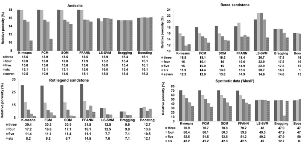
Figure 2.Relative porosity values obtained using unsupervised, supervised and ensemble classifier techniques for respective samples.
detection and surface procedure proposed by Yanowitz and Bruckstein (1989). Convergence active countours (CAC)-Sheppard is a hybrid method developed by (CAC)-Sheppard et al. (2005) which uses a combination of image enhancement, thresholding and convergence active contours. Markov ran-dom fields (MRF)-Berthod is an algorithm for supervised Baysian image classifaction using Markov random fields de-veloped by Berthod et al. (1996). The general drawback of CAC-Sheppard and MRF-Berthod methods can be attributed to long processing time caused by insufficient ground truth initialization and long processing time due to the simulated annealing technique. Jovanovic et al. (2013) proposed a seg-mentation scheme which can be performed already at the stage of sinograms. Cortina-Januchs et al. (2011) used a seg-mentation/classification technique based on a combination of clustering and artificial neural network (ANN) to segment bi-nary soil images, whereas Khan et al. (2016) used the super-vised technique least-squares support vector machine (LS-SVM) for segmentation of XCT rock images. Therefore, with the continuously, improving CT technologies and computa-tional resources, machine learning (ML) techniques can be an effective tool for segment and classify for phase segmen-tation of XCT rock images. Based on the heterogeneity of the sample the user can employ different ML techniques to ob-tain the best segmented image(s), which can be further used for simulating physical processes.
In Chauhan et al. (2016), we developed a workflow to seg-ment XCT images using unsupervised, supervised and en-semble classifier ML techniques. The focus of this study is to assess the performance and accuracy of the above mentioned ML techniques to segment rock grain, matrix and pore phases
in heterogeneous rock samples such as andesite, Berea sand-stone, Rotliegend sandstone and a synthetic sample contain-ing microporosities.
2 Experimental approach
al. (2012), using a scanning electron microscope, revealed Berea sandstone has ankerite, quartz, zircon, K feldspar and clay. The synthetic sample contained large pores, micropores and mineral grain.
Andesite volcanic rock and Rotliegend sandstone were im-aged using a custom-built XCT scanner based on the CT-ALPHA system (ProCon, Sarstedt, Germany) at the Institute for Geosciences laboratory in Mainz, Germany. The sam-ples were scanned by applying X-ray energy of 110 keV and using a prefilter of 0.3 copper. During the reconstruc-tion of the projecreconstruc-tions, a noise filter was not used. The pro-jections were radon-transformed in sinograms and thereafter converted through back projection into tomograms. These stacked tomograms resulted in 16 bit 3-D imagery, with a resulting voxel resolution of 13 and 21 µm for andesite and sandstone, respectively. Andesite required no beam harden-ing correction (BHC), whereas BHC for sandstone was done based on regression analysis using 2-D paraboloid fitting. Fi-nally, the tomograms are saved in raw format.
The Berea sandstone dataset was obtained from the GitHub FTP server (https://github.com/cageo/ Krzikalla-2012). Andrä et al. (2013) performed XCT scans at the Tomographic Microscopy and Coherent Radi-ology Experiments (TOMCAT) (Stampanoni et al., 2006) beamline at the Swiss Light Source (Paul Scherrer Institute, Villigen, Switzerland). The beam energy was tuned for best contrast at 26 keV with an exposure time of 500 ms to retrieve a magnification of factor 10 (Andrä et al., 2013). The projections were magnified by microscope optics and digitized by a high-resolution CCD camera (PCO.2000) to obtain images of dimension 1024×1024×1024 with voxel resolution of 0.74 µm. Tomographic images were reconstructed from the sinograms by applying Fourier transform spectroscopy (Marone et al., 2009) and saved in the desired file formats (Andrä et al., 2013).
2.1 Image pre-processing
Each of the 16 and 8 bit 3-D reconstructed raw images re-sulted in 20483and 10243voxels. The image filtering tech-niques such as blur, background intensity variation and con-trast were tested on all the raw images before the segmen-tation and classification algorithms were initialized. In the case of Rotliegend sandstone (21 µm), as the XCT images were noisy, a contrast filter was used to enhance the image; for other XCT images (Berea, andesite and Musli), as the resolution and contrast were sufficiently high (7.5 to 13 µm), using filters did not show any noticeable change. The follow-ing sections describe the post-processfollow-ing algorithm and how these were implemented in our image processing schemes.
3 Machine learning
The main focus of this study is to demonstrate the compu-tational performance and accuracy of the different ML al-gorithms to segment/classify different phases in XCT rock samples – i.e., to map pixels of similar values into respec-tive classes. ML algorithms rely on features; features are sets of instances which contain descriptive information based on which the ML algorithm trains it classification model and further identifies these features in an unknown dataset and groups them into respective classes, which in our case are the associated feature values of noise, rock grain, matrix and pore voxels. ML algorithms in general fall into categories of unsupervised, supervised and ensemble classifiers.
3.1 Unsupervised techniques
In the unsupervised techniquek-means (MacQueen, 1967), fuzzy c-means (FCMs) (Dunn, 1973) and self-organized maps (SOMs) (Kohonen, 1990) were used for segmentation of pore, mineral and matrix phases. The k-means cluster-ing algorithm is one of the simplest unsupervised ML al-gorithms commonly used to address the clustering problem. Thek-means algorithm through an iterative scheme calcu-lates the Euclidean distance between the data point (pixel value) and its nearest centroid (cluster). The algorithm con-verges when the mean square root error of Euclidean distance reaches minimum; that is, when no further pixel is left to be assigned to the nearest centroid (cluster). The performance of thek-means algorithm is strongly governed by the initial choice of the cluster centres. Thek-means has the tendency to terminate without identifying the global minimum of the objective function (Chauhan et al., 2016). Therefore, it is rec-ommended to run the algorithm several times to increase the likelihood that the global minimum of the objective function will be identified.
Unlikek-means, in the FCM iterative scheme each data point can be a member of multiple clusters by varying the membership function (Jain, 2010 and Jain et al., 1999). The FCM clustering procedure involves minimizing the objective function
Jfcm(Z;U;V )=
Xn j=1
Xk i=1(µij)
m x
(i) i −ck
2
S. Chauhan et al.: Phase segmentation of X-ray computer tomography rock images 1129
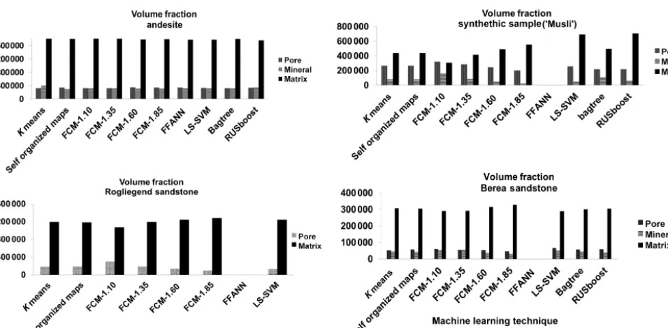
Figure 3.Total volume fraction plotted for respective samples.
FCMs can be a better choice in comparison tok-means, but it has a tendency to converge to the local minima of the objec-tive function. Therefore, it is vital to test a range of member-ship values in combination with several centroids (classes) for accurate analysis (Cannon et al., 1986).
For a detailed description of SOMs the reader is referred to Kohonen (1990) and Chauhan et al. (2016). The SOM pro-cedure uses a competitive learning process based on an ANN framework. In our context, a raw CT image is considered as an input pattern, which has to be classified. SOMs first ar-range nodes (called neurons) in one of the desired topologies (grid, hexagon or random topology, as specified by the user) and assigns random weight (values). These nodes are trained using the pixel value of the CT image(s), iteratively using the Kohonen rule (Kohonen, 1990). During this competitive learning process the difference between the nodal weight and the neighboring pixel(s) is calculated. The iterative process stops when the difference reaches a minimum. The amount of adaptation of the nodal weight to its neighboring values can be influenced and monitored using learning rate parame-terα. The nodes that do not change to its surrounding value are classed as winner nodes. These winner nodes are nothing but different classes in the segmented image.
The unsupervised algorithms were configured to perform segmentation of three to seven classes. These classes in one-dimensional feature space are the non-overlapping segments of pixel bins in a histogram. Filter-based feature vector (FV) selection (Euclidian and Manhattan distance function) were used to initialize centroids for k-means, FCMs and SOMs. In the case of FCMs different degrees of membership values [1.10 to 1.85] were tested to loosely or tightly segregate pixel
values between rock grains and matrix phase. Grid topology was chosen in the case of SOMs.
3.2 Supervised techniques
In the supervised category feed forward artificial neural net-work (FFANN) (Jain et al., 1999) and LS-SVM (Suykens and Vandewalle, 1999) were used to classify rock grains, matrix and pore phases (Chauhan et al., 2016). In general, the su-pervised algorithms rely on a classification model which has to be trained using an example set of data that represent each class.
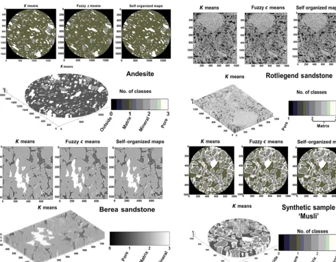
Figure 4.The top, middle and last panel show the 2-D segmented images and volume rendered plots of respective samples using unsupervised networks (andesite figure has been modified after Chauhan et al., 2016).
For LS-SVM a training dataset was created which con-tained a range of pixel values which best represented pore, mineral, matrix, cracks, trapped pores and noise regions; these pixel ranges were further labeled into different classes, which ranged from one to seven. For FFANN and LS-SVM the models were tuned using the 10 K-fold cross-validation function (repeated training and testing), and the misclassifi-cation rate was determined using mean MSE in the case of FFANN. Once the classification model reached an optimal performance threshold, it was tested on the rest of the XCT slices.
3.3 Ensemble classifier techniques
In the ensemble classifier technique RUSBoost and Bragtree algorithms are used (Seiffert et al., 2008; Breiman, 1996) to classify pore, rock grains and matrix phases (Chauhan et al., 2016). In general ensemble classifiers are a “bootstrap aggregation” of different weak classifiers. In general, weak
learn-S. Chauhan et al.: Phase segmentation of X-ray computer tomography rock images 1131
ing rate, which is a parameter from a [0.0, 1.0] control over-fitting range, was set to 0.1. Smaller values of learning rate require large numbers of weak learners to maintain a constant training error. Empirical evidence suggests that small values of learning rate favor better test error, as the constraint on the given number of weak learners maintains a constant training error.
3.4 Feature selection
In a practical rock CT segmentation/classification task, a pri-ori information representing different phases (pore, matrix, rock, cracks, trapped pores etc.) in the XCT image is given to ML algorithms for segmentation or training the classifi-cation model. The dataset used as a priori information con-tains pixel values representing different phases in the XCT image, termed feature vectors. For unsupervised k-means, FCMs and SOMs, 10 slices from a XCT images were used to develop the FVs. For FFANN 5 images out of 10 were used to train the network; for LS-SVM and ensemble based classi-fiers different subset of pixels representing the pore, mineral, matrix, cracks, trapped pore and noise regions were used as feature vectors. The total number of pixels used to train and test each ML algorithm is shown in Table 1.
3.5 Performance
Computational performance was measured in terms of the segmentation and classification speed of the ML algorithms. Tests were performed on a Windows Server 2008 R2 Stan-dard 64 bit operating system, with two six-core Intel Xeon processors, CPU (E645, 2.40 GHz) and installed memory (RAM) of 48.0 GB.
3.6 Accuracy
There is a wide set of evaluation metrics available to compare the quality of clustering and classification algorithms. For unsupervised clustering techniques accuracy can be evalu-ated intrinsically; i.e how close are the elements to each other within a cluster and how far apart from elements of other clusters (Amigó et al., 2009). Extrinsic metrics, on the other hand, are a comparison between the output of the clustering system and thegold standardusually built using human as-sessors (Amigó et al., 2009). Stehl (2002), Meilˇa (2003) and Amigó et al. (2009) proposed several types of cluster eval-uation metrics tested on different mathematical constraints. However, the appropriate metrics for cluster evaluation is nontrivial and is still a subject of discussion. In this work, we use extrinsic evaluation metrics “purity” and “entropy”, which are most commonly used for clustering problems. The idea is to identify ideal class(es), representing the “best” porosity values, and to compare the clustering algorithm.
Any supervised classification is incomplete until the as-sessment of its accuracy has been performed. The super-vised classification models are trained with a priori
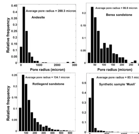
informa-Figure 5.The pore size distribution of different rock samples using a watershed technique.
tion which is almost a subset of classes under investigation. Stehman et al. (2003) pointed out the accuracy assessment of a supervised classification problem can be assessed in three different steps: (1) the design of the model, (2) the response of the designed model to obtain the true classification rate (minimum error rate) and (3) the analysis of the classified data. The most common methods used for the analysis of the classified data are confusion matrix orκ – error statis-tics introduced by Fleiss et al. (1969). For our accuracy as-sessment study we have used step 2, the response of the de-signed model, to obtain the true classification rate: namely, metrics such as MSE, ROC and 10 K-fold cross-validation for AANN, LS-SVM and ensemble classifiers, respectively.
Subsections below illustrate all the metrics used for evalu-ating unsupervised, supervised and ensemble classifiers. 3.6.1 Entropy and purity
The entropy of a class reflects how the members of thek pix-els are distributed within each class; the global quality mea-sure is by averaging the entropy of all classes:
entropy= −X j
nj
n
X
iP (i, j )×log2P (i, j ), (2) whereP (i, j )is the probability of finding an item from the categoryiin the classj, wherenj is the number of items in classj andnthe total number of items in the distribution.
Table 1.The number of pixels used for training and testing the classification model.
Type of classifiers Andesite Rotliegend sandstone
No. of training pixels No. of testing pixels No. of training pixels No. of testing pixels
K-means 31 577 290 13 681 600
Fuzzyc-means 31 577 290 13 681 600
Self-organized maps 31 577 290 13 681 600
Artificial neural networks 15 788 645 31 577 290 6 840 800 13 681 600 Least-squares support vector machine 2077 31 577 290 1511 41 943 040 Bragging and boosting 2077 31 577 290 1511 41 943 040
Type of classifiers Synthetic sample (Musli) Berea sandstone
No. of training pixels No. of testing pixels No. of training pixels No. of testing pixels
K-means 10 000 000 4 056 000
Fuzzyc-means 10 000 000 4 056 000
Self-organized maps 10 000 000 4 056 000
Artificial neural networks 5 000 000 10 000 000 20 28 000 4 056 000 Least-squares support vector machine 1655 10 000 000 1366 4 056 000 Bragging and boosting 1655 10 000 000 1366 4 056 000
Figure 6.Entropy values of unsupervised techniques plotted for respective samples.
andLthe set of classes, purity=X
i |Ci|
N maxj precision(CiLj), (3)
where the precision of a pixelsCi for a given classesLi is defined as
precision CiLj=
Ci∩Lj
|Ci|
. (4)
S. Chauhan et al.: Phase segmentation of X-ray computer tomography rock images 1133
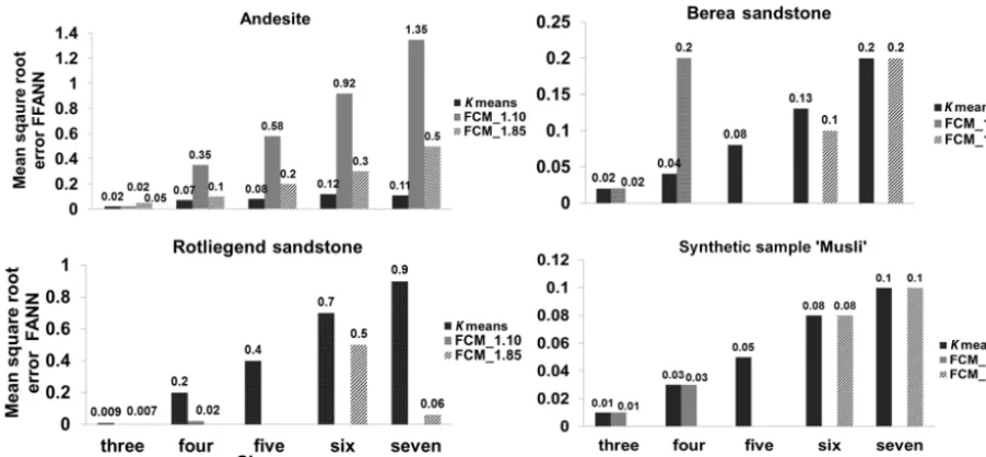
Figure 7.Mean square root error values of feed forward artificial neural network (FFANN) obtained for respective samples. FFANN was trained using segmented datasets ofk-means, fuzzyc-means with a membership function of 1.10 and 1.85
3.6.2 Mean square root error
The most commonly used error metrics to assess the accu-racy of the FFANN are the MSE, the mean square relative error (MSRE), the coefficient of efficiency (CE) and the co-efficient of determination (R2), shown in the equations be-low:
MSE=Xn i=1
Qi−Qei
2
Q2i , (5)
MSRE= Pn
i=1 Qi−Qei
2
Q2i
n , (6)
CE=1− Pn
i=n Qi−Qei
2
Pn
i=n Qi− ¯Qi
2, (7)
R2=
Pn
i=1 Qi− ¯Qi
e
Qi− ´Qi
q Pn
i=1 Qi− ¯Qi 2
Pn
i=1
e
Qi− ´Qi
2
2
, (8)
whereQei are the classified images by FFANN.Qi are the images used for training the FFANN (k-means and FCM im-ages),Q¯iis the mean of the images used for training FFANN andQ´iis the mean of the classified images To evaluate accu-racy of our FFANN model, we looked at the MSRE values. The lower the MSRE value, the higher is the accuracy of the prediction.
3.6.3 Receiver operational characteristics
Receiver operational characteristic (ROC) curves have long been used in the signal detection theory (Bradley, 1997). It is
a good way of cross-validation of classifiers’ accuracy (prob-ability of classifiers correct responseP (C)).
accuracy(1−error)= Tp+Tn
Cp+Cn
=P (C), (9)
sensitivity(1−β)=Tp
Cp
=P (Tp), (10)
specificity(1−α)=Tn
Cn
=P (n), (11) whereTpandTnare the true positive and true negative exam-ples andCpandCnare total number of true positive and true negative examples.
Probability of false positive isP (Fp)=α Probability of true positive isP (Tp)=(1−β)
The accuracy is determined by calculating the area under the curve (AUC), and the simplest was to do that is by using trapezoidal approximation.
AUC=X
i
(1−βi·1α)+ 1
2(1 (1−β)·1α)
(12) In our case the AUC was determined using the trapezoidal approximation for each exponential curve, and the values were the fraction multiplied by 100 to obtain the value in percent.
3.6.4 10 K-fold cross-validation
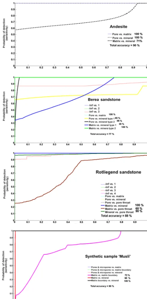
Figure 8. Receiver operational characteristic curves depicting the accuracy of the least-squares support vector machine multi-classification scheme for class four. A few curves which appear in the legend have close proximity to thexaxis and lie behind other curves and therefore are invisible.
into two segments: one used to learn or train a model and the other used to validate the model. The problem with evaluat-ing such a model is that it may demonstrate adequate predic-tion capability on the training data, but it might fail to predict future unseen data. Cross-validation is a procedure for esti-mating the generalization performance in this context.
Later, Kohavi (1995) and Dietterich (1998) investigated several approaches to estimate the accuracy of classifiers using different combinations of 10 K-fold cross-validation techniques; they recommended 10 K-fold cross-validation as one of the best cross-validation techniques, as it mitigates biases despite variances in the size of training and testing datasets.
At the onset of 10 K-fold cross-validation, the dataset is initially stratified and partitioned into 10 equal (or nearly equal) segments or folds. Subsequently 10 iterations of train-ing and validation are performed such that within each iter-ation a different fold of the data is held out for validiter-ation, while the rest of the folds are used for learning.
4 Results and discussions
4.1 Porosity and pore size distribution
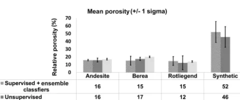
The porosities which were determined from the stack of 10 XCT slices for three to seven classes using different ML techniques are shown in the Fig. 2. The estimated porosity is the ratio between the pore phase voxels and entire sam-ple volume multiplied by 100. In general, the porosity us-ing unsupervised ML techniques agrees well for all the four samples within±1.2 % for each class. For andesite, Berea, sandstone, Rotliegend sandstone and Musli, the average esti-mated porosity sum over all classes is 15.8±2.5, 16.3±2.6, 13.4±7.4 and 48.3±13.3 %, respectively. This is in good agreement with the experimental porosity values obtained for andesite and Rotliegend sandstone using a GeoPyc pycnome-ter and Berea sandstone as reported in Andrä et al. (2013). The large standard deviation in the case of sandstone and Musli is caused by the FCM segmentation scheme. When the membership function is tightly constrained [1.10, 1.35], the segregation between pore phase voxels and pore throat vox-els is underestimated, contributing to the increase in porosity. Conversely, when the membership function is loosely con-strained [1.60, 1.85], pore throat and micropores are seg-mented as matrix phases, resulting in a decrease in porosity and increase in matrix phase, which is clearly visible in the volume fraction plot of sandstone and Musli in Fig. 3. The low standard deviation in the estimated porosity values of andesite is due to the absence of microporosity and intercon-nected pores. The pore, mineral and matrix phases are dis-tinct from each other; therefore the ML techniques have less difficulty in segmentation and classification. Figure 4 shows the segmented images using unsupervised technique and re-spective volume rendered images.
S. Chauhan et al.: Phase segmentation of X-ray computer tomography rock images 1135
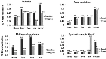
Figure 9.Accuracy of ensemble classifiers boosting and bragging calculated using 10 K-fold validation for respective samples.
Distance transform to convert the bright area into catchment basin and later watershed transformation was performed to segment the pore boundaries. Figure 5 shows the PSD and average pore radius of andesite, Berea sandstone, Rotliegend sandstone and Musli fromk-means segmented images.
4.2 Performance and accuracy analysis
Performance in the form of computational time is tabulated in Table 2. Thek-means algorithm is the fastest among all the ML techniques because segmentation of phases into different classes is based on nearest-neighborhood distance measure-ments, unlike other ML techniques (exception: FCM), where the classification is governed by classification models.
In the case of supervised techniques the computational speed is correlated with the size of the feature vector used for training the classification model and post-processing of the unknown dataset. One reason is that supervised tech-niques are based on a “single” classification model; train-ing and cross-validation of the model with a large amount of feature vectors consumes time. This can be related to the high computational time of the andesite sample using FFANN, where five slices were used to train the tion model compared to other samples where the classifica-tion model was trained using only one slice. For LS-SVM – as feature vector pixels are less than 1 % of the total pixel values for the all the samples – the training of the classifi-cation model took 1 to 10 min. The high computational time was consumed in post-processing, where a large unknown
dataset was subjected to the trained model. In the case of en-semble classifiers the post-processing of an unknown dataset took longer compared to the training of the respective (boot-strapped weak) classification schemes. As the Rotliegend sandstone is densely packed with very low porosity, it re-sulted in low contrast and a badly resolved XCT dataset. As a consequence, the individual (weak) classification mod-els required more computational time to achieve a consoli-dated, nearly accurate, well-classified result. Therefore, the processing time of Rotliegend sandstone images by ensem-ble classifiers was higher compared to other XCT samples.
Table 2.The computational time for processing 10 slices.
Machine learning techniques CPU: time (h:min:s)
Andesite Rotliegend sandstone Synthetic sample (Musli) Berea sandstone
K-means 00:15:35 00:12:04 00:10:59 00:05:33
FCM 00:29:19 00:56:03 00:42:21 00:41:05
SOM 01:07:06 1:41:47 01:11:23 00:33:32
FFANN (training usingk-means) 08:58:18 00:11:50 00:10:40 00:11:12 LS-SVM* 63:29:35 03:22:58 03:02:15 01:45:17 Bragging 05:57:05 07:32:22 12:19:40 03:51:13 Boosting 07:47:05 09:52:56 06:14:58 03:20:42:
*Open-source public library provided by the University of Leuven’s Department of Electrical Engineering (ESAT) SCD-SISTA division was used:
http://www.esat.kuleuven.be/sista/lssvmlab/.
Figure 10.Mean porosity value obtained using supervised and en-semble classifiers as well as unsupervised machine learning tech-niques.
For FFANN the accuracy was interpreted using Eqs. (6) and (8) and the MSE shown in Fig. 7. FFANN was trained using k-means and FCM and was tested on raw XCT im-ages of the respective samples. The testing dataset (3-D stack of raw images) was scaled between three and seven class values before the start of the testing cycle. In the case of Berea, Rotliegend and the synthetic sample, when the mem-bership function was tightly constrained to 1.10, FCM was able to segment pore, matrix and mineral grain phases into a maximum of three and four classes. Similarly, on a moder-ate (1.60) and loosely constrained (1.85) membership func-tion FCMs yield a maximum of five, six and seven classes, respectively. This explains the variance in the number of datasets used for validation of FFANN. The lower the MSE value, the better is the accuracy; the accuracy decreases with over-classification (for class five to six). Different settings, such as increasing the number of training slices up to five and increasing the number of neurons from 10 to 30, did not show any significant improvement in the accuracy. Among all the XCT samples, the worst accuracy was found for Rotliegend sandstone. Based on our analysis, we suggest that FFANN may not be the best-suited ML technique for clustering anal-ysis.
In the case of LS-SVM, the low variance seen in the poros-ity values up to class six, is the indication that LS-SVM is one
among the most suitable ML techniques for phase segmen-tation analysis of XCT images. As the hand-picked feature vector dataset of class four had an appropriate mix of all the phases and the desired amount of noise, it gave the best trade-off between quality and speed. Hence we show the accuracy of LS-SVM for classification of class four using the ROC curve (Metz, 1978) in Figure 8. The slope of the ROC curve gives the accuracy of classification which was computed us-ing Eq. (12). The accuracy ranges from 77 % for Berea sand-stone to 88 % for Rotliegend sandsand-stone and 90 % for andesite and Musli. Up to 100 % accuracy is achieved in discriminat-ing the pore phase with respect to mineral and matrix phases. Ensemble classifiers also show low variance in the poros-ity values as LS-SVM because of the same feature vectors used. The accuracy of the ensemble classifiers tested using the 10 K-fold cross-validation technique (Quinlan, 1996) is shown in Fig. 10. Both Bragging and Boosting classifiers where trained using the training dataset. The training dataset comprises the pixel values representing pore, mineral, ma-trix, noise phases and feature vectors. The initial growth of the leaf size was started with 5, and the corresponding weak classifiers were trained up to 1000 iterations (Breiman et al., 1996). The accuracy was determined by 10 K-fold cross-validation techniques. The best accuracy was achieved for andesite and Musli XCT (with an exception for class six) im-ages, and the worst for Rotliegend sandstone, going up to 0.56.
5 Conclusions
S. Chauhan et al.: Phase segmentation of X-ray computer tomography rock images 1137
al. (2013). The high standard deviations up to 13 % seen in the case of Musli can be attributed to the misclassification caused by ensemble classifiers at class six. This can be seen in the porosity value of Musli in Fig. 2. The feature vector set corresponding to class siz introduces noise information in the form of 73 pixels. When the training/testing was performed using feature vector up to class six, the ensemble classifiers showed high misclassification. Thereafter, when additional information on cracks and specks represented as 300 and 97 pixels is introduced as class seven (feature vector), the en-semble classifier stablizies. It is difficult to speculate why this happens.
Our analysis shows unsupervised ML techniques perform well with filter-based feature extraction techniques. In terms of computational time, k-means outperforms all the other ML techniques. Fuzzyc-means can distinguish well between pore and pore-throat boundaries, given that the membership function is loosely constrained between 1.60 and 1.85. It was found that different tuning parameters (such as differ-ent FCM membership criteria and differdiffer-ent SOM topologies and distance functions) need to be tested for the unsupervised techniques. A SOM topology “grid top” layout (neurons ar-ranged in a grid format) and a SOM Manhattan distant func-tion (sum of the absolute difference) gave consistent results, and FCM membership function within [1.35–1.85] gave con-sistent results. Low entropy values ofk-means indicate that
k-means is more accurate compared to fuzzy c-means and self-organized maps.
In the case of supervised techniques the computational time was significantly improved by reducing the training dataset of FFANNs and by careful selection of feature vector dataset for LS-SVM. Based on our analysis we conclude that FFANNs may not be best suited for clustering analysis; due to difficulty in scaling the training dataset (XCT raw files), the interpretation of clustering labels and accuracy becomes extremely difficult. Additionally, the accuracy in terms of mean square root error of the validation cycle (training and repeated testing) is largely regularized by fine and coarse scaling of the testing dataset, which may not always corre-spond to the image classification. As a consequence, there were cases where despite low accuracy (high MSE) the clas-sification performed by FFANN was good. LS-SVM, how-ever, proved to be one of the best and accurate supervised ML techniques for phase segmentation problem. However, it strongly relies on the craft with which the feature vec-tor dataset is constructed. The user has the flexibly to de-cide which phases or feature are most relevant for phase seg-mentation. The authors suggest using the histogram plot of the raw image or k-means (or any other unsupervised ML technique) as an orientation for feature vector selection. It is further recommended that the first and second class la-bels (e.g., class three and class four) should contain pre-dominantly phases such as pore, matrix, mineral and noise pixels. Consequently, other interesting feature pixels can be included. A suitable balance has to be found, such that the
classifier is not excessively trained on one particular feature and does not get stuck in local minima. Thereafter, the ROC curve validation technique is best suited for accuracy assess-ment of LS-SVM.
Ensemble classifier can be the second-best alternative to tackle phase segmentation problems as it also relies on the feature vector dataset to train the classification model; there-fore, the user has more control over the classification scheme. However, the weak learners involved in the ensemble clas-sification scheme remain as a black box to a large extent; therefore, appropriate tuning of the individual weak learners to optimize computational speed and accuracy may be cum-bersome. To have a better control over the ensemble classifi-cation scheme, and for future work, we suggest an ensemble classifier withk-means, FCMs and LS-SVM as weak learn-ers.
Acknowledgements. We thank Michael Kersten, Frieder Enzmann and his group at the Institute for Geoscience, Johannes-Gutenberg-Universität Mainz, for the high-resolution X-ray tomography measurements of andesite and Rotliegend sandstone. We thank Phillip Mielke and Achim Aretz for the fieldwork and collection of rock samples, and Heiko Andrä and her team at Fraunhofer ITWM Germany for making the synchrotron dataset of Berea sandstone freely available online.
This work is funded within the framework of the SUGAR (Sub-marine Gashydrat Ressourcen) III project by the German Federal Ministry of Education and Research (BMBF grant no. 03SX381H) and also partly supported by the DFG in the framework of the Excel-lence Initiative, Darmstadt Graduate School of ExcelExcel-lence Energy Science and Engineering (GSC 1070). The sole responsibility for the content lies with the authors.
We thank two anonymous reviewers and the editor, Steven Henkel, for their valuable comments which improved the manuscript.
Edited by: S. Henkel
Reviewed by: two anonymous referees
References
Amigó, E., Gonzalo, J., Artiles, J., and Verdejo, F.: A comparison of extrinsic clustering evaluation metrics based on formal con-straints, Inform. Retrieval, 12, 461–486, 2009.
Andrä, H., Combaret, N., Dvorkin, J., Glatt, E., Han, J., Kabel, M., Keehm, Y., Krzikalla, F., Lee, M., Madonna, C., Marsh, M., Mukerji, T., Saenger, E.H. , Sain, R., Saxena, N., Ricker, S., Wiegmann, A., and Zhan, X.: Digital rock physics benchmarks – Part I: Imaging and segmentation, Comput. Geosci., 50, 25–32, 2013.
Bradley, A. P.: The use of the area under the ROC curve in the evalu-ation of machine learning algorithms, Pattern Recogn., 30, 1145– 1159. 1997.
Breiman, L.: Bagging predictors, Mach. Lear., 24, 123–140, 1996. Berthod, M., Kato, Z., Yu, S., and Zerubia, J.: Bayesian image
clas-sification using Markov random fields, Image Vision Comput., 14, 285–295, 1996.
Cannon, R. L., Dave, J. V., and Bezdek, J.: Efficient Implementation of the Fuzzy c-Means Clustering Algorithms, IEEE T. Pattern Anal., 8, 248–255, 1986.
Chauhan, S., Rühaak, W., Khan, F., Enzmann, F., Mielke, P., Ker-sten, M., and Sass, I.: Processing of rock core microtomogra-phy images: Using seven different machine learning algorithms, Comput. Geosci., 86, 120–128, 2016.
Cortina-Januchs, M. G., Quintanilla-Dominguez, J., Vega-Corona, A., Tarquis, A. M., and Andina, D.: Detection of pore space in CT soil images using artificial neural networks, Biogeosciences, 8, 279–288, doi::10.5194/bg-8-279-2011, 2011.
De Boever, E., Varloteaur, C., Nader, F.H., Foubert, A., Békri, S., Youssef, S., and Rosenberg, E.: Quantification and prediction of the 3D pore network evolution in carbonate reserviour rocks, in: Oil & Gas Science and Technology – Rev. IFP Energies nou-velles, Vol. 67, No. 1., 161–178, 2012.
Dietterich, T. G.: Approximate statistical tests for comparing su-pervised classification learning algorithms, Neural Comput., 10, 1895–1923, 1998.
Dunn, J. C.: A Fuzzy Relative of the ISODATA Process and Its Use in Detecting Compact Well-Separated Clusters, J. Cybernetics, 3, 32–57, 1973.
Fleiss, J. L., Cohen, J., and Everitt, B. S.: Large sample standard er-rors of kappa and weighted kappa, Psychol. Bull., Psychol. Bull., 72, 323–327, doi:10.1037/h0028106, 1969.
Haykin, S.: Neural Networks: A Comprehensive Foundation, 1st Edn., Upper Saddle River, NJ, USA, Prentice Hall PTR, 1994. Hopfield, J. J.: Neural networks and physical systems with emergent
collective computational abilities, P. Natl. Acad. Sci. USA, 79, 2554–2558, 1982.
Iassonov, P., Gebrenegus, T., and Tuller, M: Segmentation of X-ray computed tomography images of porous materials: A crucial step for characterization and quantitative analysis of pore structures, Water Resour. Res., 45, W09415, doi:10.1029/2009WR008087, 2009.
Jain, A. K.: Data clustering: 50 years beyond K-means, Pattern Recogn. Lett., 31, 651–666, 2010.
Jain, A. K., Murty, M. N., and Flynn, P. J.: Data clustering: a review, ACM Comput. Surv., 31, 264–323, 1999.
Jovanovi´c, Z., Khan, F., Enzmann, F., and Kersten, M.: Simulta-neous segmentation and beam-hardening correction in computed microtomography of rock cores, Comput. Geosci., 56, 142–150, doi:10.1016/j.cageo.2013.03.015, 2013.
Khan, F., Enzmann, F., and Kersten, M.: Multi-phase classification by a least-squares support vector machine approach in tomog-raphy images of geological samples, Solid Earth, 7, 481–492, doi:10.5194/se-7-481-2016, 2016.
Kohavi, R. A.: study of cross-validation and bootstrap for accuracy estimation and model selection, in the International Joint Confer-ence on Articial IntelligConfer-ence (IJCAI), 1137–1145, 1995. Kohonen, T.: The self-organizing map, P. IEEE, 78, 1464–1480,
1990.
Larson, S. C.: The shrinkage of the coefficient of multiple correla-tion, J. Educ. Psychol., 22, 45–55, doi:10.1037/h0072400, 1931. Levenberg, K.: A method for the solution of certain problems in
least squares, Q. Appl. Math., 5, 164–168, 1944.
MacQueen, J. (Ed.): Some Methods for classification and Analy-sis of Multivariate Observations, University of California Press, 1967.
Madonna, C., Bjarne, S., Almqvist, G., and Saenger, E. H.: Digital rock physics: numerical prediction of pressure dependent ultra-sonic velocities using micro-CT imaging, Geophys. J. Int., 189, 1475–1482, 2012.
Marone, F., Hintermüller, C., McDonald., S., Abela, R., Miluljan, G., Isenegger, A., and Stampanoni, M.: X-ray tomography mi-croscope at TOMCAT, 9th International Conference on X-Ray Microscopy, J. Phys. Conf. Ser., 186, 012042, doi:10.1088/1742-6596/186/1/012042, 2009.
Marquardt, D.: An algorithm for least-squares estimation of nonlin-ear parameters, SIAM J. Appl. Math., 11, 431–441, 1963. Meilˇa, M.: Comparing clusterings by the variation of information.
Learning theory and kernel machines, Volume 2777 of the series Lecture Notes, in: Computer Science, Springer, Berlin, Heidel-berg, 173–187, doi:10.1007/b12006, 2003.
Metz, C. E.: Basic principles of ROC analysis, Seminars in nuclear medicine, 8, WB Saunders, 1978.
Oh, W. and Lindquist, B.: Image thresholding by indicator Kriging, IEEE T. Pattern Anal., 21, 590–602, 1999.
Pal, N. R: On minimum cross-entropy thresholding, Pattern Recogn., 29, 575–580, 1996.
Pal, N. R. and Pal, S. K: Entropic thresholding, Signal Processing, 16, 97–108, doi:10.1016/0165-1684(89)90090-X, 1989. Pham, T. D: Image segmentation using probabilistic fuzzy
c-means clustering, in: Image Processing, 2001. Proceedings. 2001 International Conference on, vol. 1. IEEE, 722–725, doi:10.1109/ICIP.2001.959147, 2001.
Piller, M., Schena, G., Nolich, M., Favretto, S., Raddelli, F., and Rossi, E.: Analysis of Hydraulic Permeability in Porous Media: From High Resolution X-ray Tomography to Direct Numerical Simulation, in: Transp Porous Med 80, 57–78, 2009.
Quinlan, J. R.: Bagging, boosting, and c4.5, in: Proceedings of the Thirteenth National Conference on Artifcial Intel ligence, AAAI/MIT Press, 725–730, 1996.
Rabbani, A., Jamshidi, S., and Salehi, S.: An automated sim-ple algorithm for realistic pore network extraction from micro-tomography Images, J. Petrol. Sci. Eng., 123, 164–171, 2014. Rosin, P. L.: Unimodal thresholding. Pattern recognition, 34, 2083–
2096, doi:10.1016/S0031-3203(00)00136-9, 2001.
Seiffert, C., Khoshgoftaar, T., Van Hulse, J., and Napolitano, A.: RUSBoost: Improving classification performance when training data is skewed, ICPR 2008, 19th International Conference on Pattern Recognition, 1–4, 2008.
Sheppard, A. P., Sok, R. M., and Averdunk, H.: Improved pore net-work extraction methods, in: International Symposium of the So-ciety of Core Analysts, 21–25, 2005.
S. Chauhan et al.: Phase segmentation of X-ray computer tomography rock images 1139
Stehman, S. V. and Czaplewski, R. L. Introduction to special issue on map accuracy, Environ. Ecol. Stat., 10, 301–308, 2003. Strehl, A.: Relationship-based Clustering and Cluster Ensembles
for High-dimensional Data Mining, PhD thesis, The University of Texas at Austin, 2002.
Sund, T. and Eilertsen, K.: An algorithm for fast adaptive image binarization with applications in radiotherapy imaging, IEEE T. Med. Imaging, 22, 22–28, 2003.
Suykens, J. A. and Vandewalle, J.: Least Squares Support Vector Machine Classifiers, Neural Process. Lett., 9, 293–300, 1999. Yanowitz, S. D. and Bruckstein, A. M.: A new method for image
segmentation, Comput. Vision Graph., 46, 82–95, 1989. Zack, G. W., Rogers, W. E., and Latt, S. A.: Automatic