A probabilistic framework for the cover effect in bedrock erosion

https://doi.org/10.5194/esurf-5-311-2017 © Author(s) 2017. This work is distributed under the Creative Commons Attribution 3.0 License.

A probabilistic framework for the cover effect

in bedrock erosion

Jens M. Turowski1and Rebecca Hodge2

1_{Helmholtzzentrum Potsdam, German Research Centre for Geosciences GFZ, Telegrafenberg,}

14473 Potsdam, Germany

2_{Department of Geography, Durham University, Durham, DH1 3LE, UK}

Correspondence to:Jens M. Turowski ([email protected])

Received: 23 November 2016 – Discussion started: 12 December 2016 Revised: 9 May 2017 – Accepted: 19 May 2017 – Published: 20 June 2017

Abstract. The cover effect in fluvial bedrock erosion is a major control on bedrock channel morphology and

long-term channel dynamics. Here, we suggest a probabilistic framework for the description of the cover effect that can be applied to field, laboratory, and modelling data and thus allows the comparison of results from different sources. The framework describes the formation of sediment cover as a function of the probability of sediment being deposited on already alluviated areas of the bed. We define benchmark cases and suggest physical interpretations of deviations from these benchmarks. Furthermore, we develop a reach-scale model for sediment transfer in a bedrock channel and use it to clarify the relations between the sediment mass residing on the bed, the exposed bedrock fraction, and the transport stage. We derive system timescales and investigate cover response to cyclic perturbations. The model predicts that bedrock channels can achieve grade in steady state by adjusting bed cover. Thus, bedrock channels have at least two characteristic timescales of response. Over short timescales, the degree of bed cover is adjusted such that the supplied sediment load can just be transported, while over long timescales, channel morphology evolves such that the bedrock incision rate matches the tectonic uplift or base-level lowering rate.

1 Introduction

Bedrock channels are shaped by erosion caused by count-less impacts of the sediment particles they carry along their bed (Beer and Turowski, 2015; Cook et al., 2013; Sklar and Dietrich, 2004). There are feedbacks between the evolv-ing channel morphology, the bedload transport, and the hy-draulics (e.g. Finnegan et al., 2007; Johnson and Whipple, 2007; Wohl and Ikeda, 1997). Impacting bedload particles driven forward by the fluid forces erode and therefore shape the bedrock bed. In turn, the morphology of the channel de-termines the pathways of both sediment and water, and the forces which the latter exerts on the former, and thus sets the stage for the entrainment and deposition of the sediment (Hodge and Hoey, 2016). Sediment particles play a key role in this erosion process; they provide the tools for erosion and also determine where bedrock is exposed such that it can be

worn away by impacting particles (Gilbert, 1877; Sklar and Dietrich, 2004).

sediment cover under flood conditions is currently unknown and the assumption that the cover distribution at low flow is representative of that at high flow may not be justified (cf. Beer et al., 2016; Turowski et al., 2008).

The most commonly used function to describe the cover effect is the linear decline (Sklar and Dietrich, 1998), which is the simplest function connecting the steady-state endmem-bers of an empty bed when relative sediment supplyQ∗_s =0 and full cover whenQ∗_s =1:

A∗=

1−Q∗_s for Q∗_s <1

0 otherwise. (1)

In contrast, the exponential cover function arises under the assumption that particle deposition is equally likely for each part of the bed, whether it is covered or not (Turowski et al., 2007).

A∗=

e−Q∗s _{for Q}∗

s <1

0 otherwise. (2)

Here,eis the base of the natural logarithm.

Hodge and Hoey (2012) obtained both the linear and the exponential functions using a cellular automaton (CA) model that modulated grain entrainment probabilities by the number of neighbouring grains. However, consistent with laboratory flume data, the same model also produced other behaviours under different parameterizations. One alternative behaviour is runaway alluviation, which was attributed by Chatanan-tavet and Parker (2008) to the differing roughness of bedrock and alluvial patches. Due to a decrease in flow velocity, an increase in surface roughness, and differing grain geometry, the likelihood of deposition is higher over bed sections cov-ered by alluvium compared to smooth, bare bedrock sections (Hodge et al., 2011). This can lead to rapid alluviation of the entire bed once a minimum fraction has been covered. The relationship between sediment flux and cover is also af-fected by the bedrock morphology; flume experiments have demonstrated that on a non-planar bed, the location of sedi-ment cover is driven by bed topography and hydraulics (e.g. Finnegan et al., 2007; Inoue et al., 2014). Johnson and Whip-ple (2007) observed that stable patches of alluvium tend to form in topographic lows such as potholes and at the bottom of slot canyons, whereas Hodge and Hoey (2016) found that local flow velocity also controls sediment cover location.

The relationship between roughness, bed cover, and in-cision was explored in a number of recent numerical mod-elling studies. Nelson and Seminara (2011, 2012) were one of the first to model the impact that the differing roughness of bedrock and alluvial areas has on sediment patch stabil-ity. Zhang et al. (2015) formulated a macro-roughness cover model, in which sediment cover is related to the ratio of sediment thickness to bedrock macro-roughness. Aubert et al. (2016) directly simulated the dynamics of particles in a turbulent flow and obtained both linear and exponential cover functions. Johnson (2014) linked sediment transport

and cover to bed roughness in a reach-scale model. Using a model formulation similar to that of Nelson and Semi-nara (2011), Inoue et al. (2016) reproduced bar formation and sediment dynamics in bedrock channels. All of these studies used slightly different approaches and mathematical formu-lations to describe alluvial cover, making a direct comparison difficult.

Over timescales including multiple floods, the variabil-ity in sediment supply is also important (e.g. Turowski et al., 2013). Lague (2010) used a model formulation in which cover was written as a function of the average sediment depth to upscale daily incision processes to long timescales. He found that over the long term, cover dynamics are largely in-dependent of the precise formulation on the process scale and are rather controlled by the magnitude–frequency distribu-tion of discharge and sediment supply. Using the CA model of Hodge and Hoey (2012), Hodge (2017) found that, when sediment supply was very variable (alternating large pulses with no sediment supply), the amount of sediment cover was primarily determined by the recent supply history, rather than by the relationships identified under constant sediment sup-ply.

So far, it has been somewhat difficult to compare and dis-cuss the different cover functions obtained from theoretical considerations, numerical models, and experiments, since a unifying framework and clear benchmark cases have been missing. Here, we propose such a framework and develop type cases linked to physical considerations of the flow hy-draulics and sediment erosion and deposition. We show how this framework can be applied to data from a published model (Hodge and Hoey, 2012). Furthermore, we develop a reach-scale erosion–deposition model that allows the dy-namic modelling of cover and prediction of steady states. Thus, we clarify the relationship between cover, deposited mass, and relative sediment supply. As part of this model framework, we investigate the response time of a channel to a change in sediment input, which we illustrate using data from a natural channel.

2 A probabilistic framework

2.1 Development

Here we build on the arguments put forward by Turowski et al. (2007) and Turowski (2009). Consider a bedrock bed on which sediment particles are distributed. We can view the deposition of each particle as a random process, and each area element on the bed surface can be assigned a probability for the deposition of a particle. When assuming that a given number of particles are distributed on the bed, the mean be-haviour of the exposed areaA∗ can be calculated from the following equation (Fig. 1):

Figure 1.Cartoon illustration of a bed partially covered by sedi-ment. For purpose of illustration, the bed is divided into a square raster, with each pixel of the size of a single grain. For a given number of particles in the area of the bed of interest, the exposed area fraction of the bed is dependent on the distribution of particles. Grains that sit on top of other grains do not contribute to cover. The probability that a new grain is deposited on uncovered bed is given byP (Eq. 3).

P is the probability that a given particle is deposited on the exposed part of the bed, which here is a function of the frac-tion of exposed area (A∗) and a dimensionless mass of par-ticles on the bed per area (M_s∗, explained below), but which can be expected to also be a function of the relative sedi-ment supply, the bed topography and roughness, the particle size, the local hydraulics, or other control variables.M_s∗is a dimensionless mass equal to the total mass of the particles residing on the bed per area, which is suitably normalized. A suitable mass for normalization is the minimum mass re-quired to cover a unit area,M0, as will become clear later.

The minus sign is introduced because the fraction of the ex-posed area reduces asM_s∗increases. As most previous rela-tionships are expressed in terms of relative sediment supply Q∗_s, the relation ofM_s∗toQ∗_s will be discussed later.

We can make some general statements aboutP. First,P is defined for the range 0≤A∗≤1 and undefined elsewhere. Second, P takes values between 0 and 1 for 0≤A∗≤1. Third,P(A∗=0)=0 andP(A∗=1)=1. Note thatP is not a distribution function and therefore does not need to inte-grate to 1. Neither does it have to be continuous and differ-entiable everywhere.

For purpose of illustration, we will next discuss two simple forms of the probability functionP that lead to the linear and exponential forms of the cover effect. First, consider the case that all particles are always deposited on exposed bedrock. In this case, formally, to keep with the conditions stated above, we defineP =1 for 0< A∗≤1 andP =0 forA∗=0. Thus, we can write

dA∗= −dM_s∗ for 0< A∗≤1

dA∗=0 for A∗=0 . (4)

Integrating, we obtain

A∗= −M_s∗+C, (5)

where the constant of integration C is found to equal 1 by using the condition A∗(M_s∗=0)=1. Thus, we obtain

a linear cover function. Note that the linear cover function gives a theoretical lower bound for the amount of cover: it arises when all available sediment always falls on uncov-ered ground, and thus no additional sediment is available that could facilitate quicker alluviation. In essence, this is a mass conservation argument. Now it is obvious whyM0is a

conve-nient way to normalize: in plots ofA∗againstM_s∗, we obtain a triangular region bounded by the points [0,1], [0,0], and [1,0] in which the cover function cannot exist (Fig. 2).

Similarly to above, if we set P to a constant value, k, smaller than 1 for 0< A∗≤1, we obtain

A∗=1−kM_s∗. (6)

It is clear that the assumption ofP =kis physically unre-alistic because it implies that the probability of deposition on exposed ground is independent of the amount of uncovered bedrock. Especially whenA∗is close to 0, it seems unlikely that, say, 90 % of the sediment always falls on uncovered ground. A more realistic assumption is that the probability of deposition on uncovered ground is independent of loca-tion and other possible controls but is equal to the fracloca-tion of exposed area; i.e.P =A∗. In a probabilistic sense, this is also the simplest plausible assumption one can make. Then

dA∗= −A∗dM_s∗, (7)

giving upon integration

A∗=e−Ms∗_{. (8)}

deposition on already covered bed is increased in comparison to the benchmark case.

A simple functional form that can be used to take into ac-count either one of these two effects is a power law depen-dence ofP onA∗, taking the formP =A∗α(Fig. 2a). Then, the cover function becomes (Fig. 2b)

A∗= 1−(1−α)M_s∗ 1

1−α_{. (9)}

Here, the probability of deposition on uncovered ground is increased in comparison to the benchmark exponential case if 0< α <1 and decreased ifα >1.

A convenient and flexible way to parameterizeP(A∗) in general is the cumulative version of the Beta distribution, given by

P A∗=B A∗;a, b. (10)

Here,B(A∗;a, b) is the regularized incomplete Beta func-tion with two shape parametersaandb, which are both real positive numbers, defined by

B A∗;a, b= RA∗

0 ya

−1_(1−y)b−1_dy

R1 0ya

−1_(1−y)b−1_dy . (11)

Here, y is a dummy variable. With suitable choices for a and b, cover functions resembling the exponential (a= b=1), the linear form (a=0,b >0), and the power law form (aborab) can be retrieved. Wavy functions are also a possibility (Fig. 3); thus, both of the roughness effects de-scribed above can be modelled in a single scenario. Unfortu-nately, the integral necessary to obtainA∗(M_s∗) does not give a closed-form analytical solution and needs to be computed numerically.

In principle, a suitable function P could also be defined to account for the influence of bed topography on sediment deposition. Such a function is likely dependent on the details of the particular bed, hydraulics, and sediment flow paths in a complex way and needs to be mapped out experimentally.

2.2 Example of application using model data

To illustrate how the framework can be used, we apply it to data obtained from the CA model developed by Hodge and Hoey (2012). The CA model reproduces the transport of individual sediment grains over a smooth bedrock surface. In each time step, the probability of a grain being entrained is a function of the number of neighbouring grains. If five or more of the eight neighbouring cells contain grains, then the grain has a probability of entrainment pc; otherwise it

has the probability pi. In most model runs pc was set to a

value less than that ofpi, thus accounting for the impact of

sediment cover in decreasing local shear stress (through in-creased flow resistance) and increasing the critical entrain-ment shear stress for grains (via lower grain exposure and

increased pivot angles). Thus, in the model, grain scale dy-namics of entrainment are varied by adjusting the values of piandpc. This has a direct effect on the reach-scale

distri-bution of cover, which is captured by ourP function (Eq. 3). The model is run with a domain that is 100 cells wide by 1000 cells long, with each cell having the same area as a grain. Up to four grains can potentially be entrained from each cell in a time step, limiting the maximum sediment flux. In each time step random numbers and the probabilities are used to select the grains that are entrained, which are then moved a step length of 10 cells downstream and deposited. Model results are insensitive to the step length. A fixed num-ber of grains are also supplied to the upstream end of the model domain. A smoothing algorithm is applied to prevent unrealistically tall piles of grains developing in cells if there are far fewer grains in adjacent cells. After around 500 time steps the model typically reaches a steady-state condition in which the number of grains supplied to and leaving the model domain are equal. Sediment cover is measured in a down-stream area of the model domain and is defined as grains that are not entrained in a given time step. Consequently grains that are deposited in one time step and entrained in the fol-lowing one do not contribute to the sediment cover, and so the model implicitly incorporates the effect of local sediment cover on grain deposition.

Model runs were completed with six different combina-tions ofpiandpc: 0.95/0.95, 0.95/0.75, 0.75/0.10, 0.75/0.30,

0.30/0.30, and 0.95/0.05. These combinations were selected to cover the range of relationships between relative sediment supply Q∗_s and the exposed bed fraction A∗ observed by Hodge and Hoey (2012). For each pair ofpiandpc, model

runs were completed with at least 20 different values ofQ∗_s in order to quantify the model behaviour.

Cover bed fraction and total mass on the bed produced by the model were converted using Eq. (3) into the new proba-bilistic framework (Fig. 4). The derivative was approximated by simple linear finite differences, which, in the case of run-away alluviation, resulted in a non-continuous curve due to large gradients. The exponential benchmark (Eq. 8) is also shown for comparison. The different model parameteriza-tions produce results in which the probability of deposition on bedrock is both more and less likely than in the baseline case, with some runs showing both behaviours. Cases where the probability is more than the baseline case (i.e. grains are more likely to fall on uncovered areas) are associated with runs in which grains in clusters are relatively immo-bile. These runs are likely to be particularly affected by the smoothing algorithm that acts to move sediment from allu-viated to bedrock areas. All model parameterizations predict greater bed exposure for a given normalized mass than is pre-dicted by a linear cover relationship (Fig. 3b). Runs with rel-atively more immobile cluster grains have a lower exposed fraction for the same normalized mass. Runs with low values ofpiandpcseem to lead to behaviour in which cover is more

val-0.0 0.2 0.4 0.6 0.8 1.0 0.0

0.2 0.4 0.6 0.8 1.0

0.0 0.2 0.4 0.6 0.8 1.0

0.0 0.2 0.4 0.6 0.8 1.0

Linear cover model (P=1) Alpha = 0.1

Alpha = 0.5

Exponential cover model Alpha = 2

Alpha = 5

P

robabi

lit

y of

inc

reas

ing c

ov

er

P

Exposed bed fraction A*

(b)

E

xp

os

ed

b

ed

fr

ac

tio

n

A

*

Stationary sediment mass M*

s

(a)

Figure 2.(a)Various examples for the probability functionP as a function of bedrock exposureA∗.(b)Corresponding analytical solutions for the cover function betweenA∗and dimensionless sediment massM_s∗using Eqs. (6), (7), and (9). Grey shading depicts the area where the cover function cannot run due to conservation of mass.

0.0 0.2 0.4 0.6 0.8 1.0 0.0

0.1 0.2 0.3 0.4 0.5 0.6 0.7 0.8 0.9 1.0

0.0 0.2 0.4 0.6 0.8 1.0 0.0

0.2 0.4 0.6 0.8 1.0

0.0 0.2 0.4 0.6 0.8 1.0 0.0

0.2 0.4 0.6 0.8 1.0

0.0 0.2 0.4 0.6 0.8 1.0 0.0

0.1 0.2 0.3 0.4 0.5 0.6 0.7 0.8 0.9 1.0

E

xpos

ed bed f

rac

tion

A

*

a=b=0.1 a=0.1, b=0.2 a=0.2, b=0.1

P

robabi

lit

y of

inc

reas

ing c

ov

er

P a=b=0.1 _{a=0.1, b=0.2} a=0.2, b=0.1

P

robabi

lit

y of

inc

reas

ing c

ov

er

P

Exposed bed fraction A* a=b=0.1

a=b=0.5 a=b=1 a=b=2 a=b=10

E

xpos

ed bed f

rac

tion

A

*

Stationary sediment mass M* s a=b=0.1

a=b=0.5 a=b=1 a=b=2 a=b=10

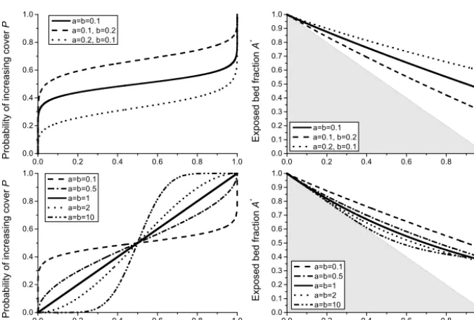
Figure 3.Examples for the use of the regularized incomplete Beta function (Eq. 11) to parameterizeP, using various values for the shape parametersaandb. The choicea=b=1 gives a dependence that is equivalent to the exponential cover function. Grey shading depicts the area where the cover function cannot run due to conservation of mass.

ues, it is less likely. However, these are complex interactions and it is difficult to generalize the model behaviour.

3 Cover development in time and space

3.1 Model derivation

Previous descriptions of the cover effect relate the exposed fraction of the bed to the relative sediment supplyQ∗_s (see Eqs. 1 and 2). In this section, we derive a model to clarify the

relationship between the exposed fraction,Q∗_s, andMs and

Tur-0 1 2 3 4 0.0

0.2 0.4 0.6 0.8 1.0

0.0 0.2 0.4 0.6 0.8 1.0 0.0

0.2 0.4 0.6 0.8 1.0

Ex

po

sed

bed

fr

act

ion

A

*

Stationary sediment mass Ms*

0.3/0.3 0.95/0.95 0.95/0.75 0.75/0.3 0.95/0.05 0.75/0.1 Exponential (Eq. 9)

Pr

obab

ilit

y

of

in

cr

ea

si

ng

co

ve

r

P

Exposed bed fraction A*

Figure 4.Probability functionsP and cover function derived from data obtained from the model of Hodge and Hoey (2012). The grey dashed line shows the exponential benchmark behaviour. Grey shading depicts the area where the cover function cannot run due to conservation of mass. The legend gives values of the probabilities of entrainmentpiandpcused for the runs (see text).

owski, 2009). In our system, we consider two separate mass reservoirs within a control volume. The first reservoir con-tains all particles in motion, the total mass per bed area of which is denoted byMm, while the second reservoir contains

all particles that are stationary on the bed, the total mass per bed area of which is denoted byMs. The reservoirs exchange

mass by entrainment and deposition; i.e. when a stationary particle is entrained it becomes mobile and when a mobile particle is deposited, it becomes stationary. In addition to Eq. (3), we then need three further equations: one to con-nect the rate of change in mobile mass to the sediment flux in the flume and one each to describe mass conservation in the two reservoirs. Instead of the common approach tracking the height of the sediment over a reference level, as is done in the classic mass conservation in fluvial systems, the Exner equation (e.g. Paola and Voller, 2005), we use the total sed-iment mass on the bed as a variable. Mobile sedsed-iment mass is supplied from upstream (1in), leaves in the downstream direction (1out), and can be exchanged between the station-ary and the mobile mass reservoirs by entrainment (Etot) and

deposition (Dtot) (Fig. 5). The latter two parameters describe

the exchange of particles between reservoirs; in the single-reservoir Exner equation these terms are not needed. It is clear that for the problem at hand the choice of total mass or volume as a variable to track the amount of sediment in the reach of interest is preferable to the height of the alluvial cover, since necessarily, when cover is patchy, the height of the alluvium varies across the bed.

The difference form of the mass balance for the mobile sediment is then given by (cf. Fig. 5)

1Mm=(1in−1out+Etot−Dtot)1t. (12)

Here,1Mmis the change in mobile sediment mass and1t

is a change in time. As the length of a time step is reduced to 0, a continuous version of Eq. (12) is obtained, which reads

∂Mm

∂t = −

∂qs

∂x +E−D. (13)

Here,xis the coordinate in the streamwise direction,tthe time, andqsthe sediment mass transport rate per unit width,

Stationary massM_s

Mobile massM_m

E

D

∆

in

∆

out

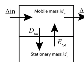
Figure 5.Sediment dynamics at the bed are modelled by two reser-voirs for stationary and mobile mass, which can exchange material by entrainment (Etot) and deposition (Dtot). Sediment mass can be supplied from upstream (1in) and can leave in the downstream di-rection (1out).

whileE is the mass entrainment rate per bed area andDis the mass deposition rate per bed area. Similarly, in the mass balance for the stationary mass reservoir, the rate of change of the stationary sediment massMsin time is the difference

of the deposition rateDand the entrainment rateE:

∂Ms

∂t =D−E. (14)

It is useful to work with dimensionless variables by defin-ing t∗=t /T and x∗=x/L, where T and L are suitable time and length scales, respectively. The dimensionless mo-bile mass per bed areaM_m∗ is equal toMm/M0, and Eq. (13)

becomes

∂M_m∗ ∂t∗ = −

∂q_s∗ ∂x∗+E

∗₋

D∗. (15)

Here,

q_s∗= T LM0

qs. (16)

The dimensionless entrainment and deposition rates,E∗ andD∗, are equal toT E/M0andT D/M0, respectively.

written as

∂M_s∗ ∂t∗ =D

∗₋

E∗. (17)

We also need sediment entrainment and deposition func-tions. The entrainment rate needs to be modulated by the availability of sediment on the bed. IfM_s∗is equal to 0, no material can be entrained. A plausible assumption is that the maximal entrainment rate,E_max∗ , is equal to the transport ca-pacity.

E_max∗ =q_t∗ (18)

Here, q_t∗ is the dimensionless mass transport capacity, which is related to the transport capacity per unit width qt

by a relation similar to Eq. (16). To first order, the rate of change in entrainment rate, dE, is proportional to the differ-ence ofEmaxandEand to the rate of change in mass on the

bed.

dE∗= E_max∗ −E∗

dM_s∗= q_t∗−E∗

dM_s∗ (19)

Integrating, we obtain

E∗=E∗_max1−e−Ms∗

=1−e−Ms∗

q_t∗. (20)

Here, we used the conditionE∗(M_s∗=0)=0 to fix the in-tegration constant toE∗_max. As required, Eq. (20) approaches E_max∗ asM_s∗ goes to infinity and is equal to 0 whenM_s∗ is equal to 0. Using a similar line of argument and by assuming the maximum deposition rate to be equal toq_s∗, we arrive at an equation for the deposition rateD∗.

D∗=1−e−Mm∗

q_s∗ (21)

WhenM_m∗ is small, then the amount that can be deposited is limited by M_m∗. If Mm∗is large, then deposition is

lim-ited by sediment supply. Substituting Eqs. (20) and (21) into Eq. (17), we obtain

∂M_s∗(x∗, t∗)

∂t∗ =D

∗₋

E∗= (22)

1−e−Mm(∗ x∗,t∗)q_s∗ x∗, t∗−1−e−Ms∗(x∗,t∗)

q_t∗ x∗, t∗.

Note thatq_s∗/q_t∗=Q∗_s. The equation for the mobile mass (Eq. 14) becomes

∂M_m∗(x∗, t∗)

∂t∗ = −

∂q_s∗ ∂x∗−

1−e−Mm(∗ x∗,t∗)

q_s∗ x∗, t∗

(23)

+1−e−Ms∗(x∗,t∗)

q_t∗ x∗, t∗.

Finally, the sediment transport rate needs to be propor-tional to the mobile sediment mass times the downstream sediment speedU, and we can write

q_s∗ x∗, t∗=U∗ x∗, t∗M_m∗ x∗, t∗. (24)

Here

U∗=T

LU. (25)

After incorporating the original equation betweenA∗and M_s∗ (Eq. 3), the system of four differential Eqs. (3), (22), (23) and (24) contains four unknowns: the downstream gradi-ent in the sedimgradi-ent transport rate∂q_s∗/∂x∗, the exposed frac-tion of the bedA∗, the non-dimensional stationary massM_s∗, and the non-dimensional mobile massM_m∗, while the non-dimensional transport capacityq_t∗ and the non-dimensional downstream sediment speedU∗are input variables andP is a externally specified function. In addition, sediment input q_s∗needs to be specified as an upstream boundary condition and initial values for the mobile massM_m∗, and the stationary massM_s∗need to be specified everywhere.

3.2 Time-independent solution

In this chapter, we discuss the steady solution to the system of equations and thus clarify the relationship between cover, stationary sediment mass, sediment supply, and transport ca-pacity. Setting the time derivatives to 0, we obtain a time-independent solution, which links the exposed area directly to the ratio of sediment transport rate to transport capacity. From Eq. (23) it follows that in this case, the entrainment rate is equal to the deposition rate, and we obtain

1−e−Mm∗

q∗

s =

1−e−Ms∗

q_t∗. (26)

Here, the bar over the variables denotes their steady-state value. Substituting Eq. (24) to eliminateM∗

mand solving for

M∗

s gives

M∗

s = −ln

1−1−e−qs∗/U∗ q∗

s

q_t∗

(27)

= −ln

1−

1−e− q_t∗ U∗Q∗s

Q∗

s

.

Note that we assume here that sediment cover is only de-pendent on the stationary sediment mass on the bed, and we thus neglect grain–grain interactions known as the dynamic cover (Turowski et al., 2007). In analogy to Eq. (24), we can write

q_t∗=U∗M₀∗. (28)

Here,M₀∗ is a characteristic dimensionless mass that de-pends on hydraulics and therefore implicitly on transport capacity (which should not be confused with the minimum mass necessary to fully cover the bedM0). When sediment

transport rate equals transport capacity, thenM₀∗is equal to the mobile mass of sediment normalized by the reference massM0. It can be viewed as a proxy for the transport

The mobile mass can then, in general, be written as follows (cf. Turowski et al., 2007), remembering that the relative sed-iment supplyQ∗_s =1 when supply is equal to capacity:

M_m∗ =M₀∗Q∗_s. (29)

If we use the exponential cover function (Eq. 8) with Eqs. (27), (28), and (29), we obtain

A∗ _=1−1−e−q∗ s/U∗

q∗

s

q_t∗ =1−

1−e− q_t∗ U∗Q∗s

Q∗

s

=1−

1−e−M∗0Q∗s

Q∗

s. (30)

Similarly, equations can be found for the other analytical solutions of the cover function. For the linear case (Eq. 6), we obtain

A∗_=1+lnn_1−1−e−M₀∗Q∗ s

Q∗

s

o

. (31)

For the power law case (Eq. 9), we obtain

A∗₌h_{1+(1−α) ln}n_1−1−e−M₀∗Q∗ s

Q∗

s

oi_1−α1

. (32)

The exponential cover function essentially leads to a com-bined linear and exponential relation betweenA∗_andQ∗

s.

In-stead of a linear decline as in the original linear cover model (Eq. 1) or a concave-up relationship as in the original expo-nential model (Eq. 2), the function is convex-up for all solu-tions (Fig. 6). AdjustingM₀∗shifts the lines: decreasingM₀∗ leads to a delayed onset of cover and vice versa. The former result arises because a lower M₀∗ means that the sediment flux is conveyed through a smaller mass moving at a higher velocity. The original linear cover function (Eq. 1) can be re-covered from the exponential model with a high value ofM₀∗, since the exponential term quickly becomes negligible with increasingQ∗

s and the linear term dominates (Fig. 6c). Note

that for the linear (Eq. 5) and the power law cases (Eq. 9), high values ofM₀∗may giveA∗_{=0 forQ}∗

s <1 (Fig. 6b, d),

which is consistent with the concept of runaway alluviation. Using the Beta distribution to describe P, a numerical so-lution is necessary, but a wide range of steady-state cover functions can be obtained (Fig. 7). By varying the value of M₀∗, an even wider range of behaviours can be obtained.

The previous analysis shows that steady-state cover is con-trolled by the characteristic dimensionless mass M₀∗, which is equal to the ratio of dimensionless transport capacity and particle speed (Eq. 28). In the following, we relate M₀∗ to hydraulic variables and argue that it is, in general, not a con-stant. ConvertingM₀∗to dimensional variables, we can write

M₀∗= q

∗

t

U∗ = qt

M0U

. (33)

The minimum mass necessary to completely cover the bed per unit area,M0, can be estimated assuming a single layer

of closely packed spherical grains residing on the bed (cf. Turowski, 2009), giving

M0=

π ρsD50

3 √

3 . (34)

Here,ρs is the sediment density and D50 is the median

grain size. We use equations derived by Fernandez-Luque and van Beek (1976) from flume experiments that describe transport capacity and particle speed as a function of bed shear stress (see also Lajeunesse et al., 2010, and Meyer-Peter and Mueller, 1948, for similar equations):

qt=5.7

ρsρ

(ρs−ρ)g

_τ

ρ−

τc

ρ 3/2

, (35)

U=11.5 _τ

ρ 1/2

−0.7 _τ

c

ρ 1/2!

. (36)

Here,τc is the critical bed shear stress for the onset of

bedload motion,gis the acceleration due to gravity, andρis the water density. Combining Eqs. (34), (35), and (36) to get an equation forM₀∗gives

M₀∗=3 √

3 2π

(θ−θc)3/2

θ1/2_−0.7θ1/2 c

=3 √

3θc

2π

(θ/θc−1)3/2

(θ/θc)1/2−0.7

. (37)

Here, the Shields stressθ=τ/(ρs−ρ)gD50, andθcis the

corresponding critical Shields stress, and we approximated 5.7/11.5=0.496 with 1/2 (compare to Eqs. 35, 36). At high θ, when the threshold can be neglected, Eq. (37) reduces to a linear relationship betweenM₀∗andθ. Near the threshold, M₀∗is shifted to lower values asθcincreases (Fig. 8). The

sys-tematic variation ofU∗with the hydraulic driving conditions (Eq. 36) implies that the cover function evolves differently in response to changes in sediment supply and transport capac-ity. For a first impression, by comparing Eqs. (35) and (36), we assume that particle speed scales with transport capacity raised to the power of one-third (Fig. 9).

3.3 Temporal evolution of cover within a reach

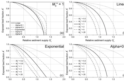
Figure 6.Analytical solutions at steady state for the exposed fraction of the bed (A∗) as a function of relative sediment supply (Q∗, cf. Fig. 2).(a)Comparison of the different solutions, keepingM₀∗constant at 1.(b)VaryingM₀∗for the linear case (Eq. 31).(c)VaryingM₀∗for the exponential case (Eq. 30).(d)VaryingM₀∗for the power law case withα=0.1 (Eq. 32).

0.0 0.5 1.0 1.5

0.0 0.2 0.4 0.6 0.8 1.0

E

xpos

ed bed f

rac

tion

A

*

Relative sediment supply Q* s

a=b=0.1 a=b=0.5 a=b=1 a=b=2 a=b=10 a=0.1,b=0.2 a=0.2,b=0.1

Figure 7.Steady-state solutions using the Beta distribution to pa-rameterizeP (Eq. 10) for a range of parametersaandband using

M₀∗=1 (cf. Fig. 3). The solutions were obtained by iterating the equations to a steady state, using initial conditions ofA∗=1 and

M_m∗=M_s∗=0.

boundary conditions. For example, during a flood event, both transport capacity and sediment supply change over time. If these changes are slow in comparison to the response time of cover, the bed cover state can essentially keep up with the imposed changes at all times, and therefore steady-state

equations (Sect. 3.2) can be used to calculate its evolution. In contrast, if the imposed change is rapid in comparison to the response time, cover may lag behind, and an approach that resolves cover as a dynamic variable is necessary. This may, for example, be important when studying the erosional be-haviour of channels in response to floods (see Lague, 2010; Turowski et al., 2013). Unfortunately, a general analytical so-lution is not possible, but results can be obtained for special cases. We first derive analytical solutions for the response time for a reach without upstream sediment supply and for a system responding to small perturbations in sediment supply or transport capacity (Sect. 3.3.1) and discuss the system be-haviour (Sect. 3.3.2). Finally, we apply the concepts to data from a flood in a natural river and demonstrate that, for this specific case, because of the response times, the steady-state relations do not capture cover behaviour.

3.3.1 System timescales

First, consider a reach without upstream sediment supply; i.e. q_s∗=0. Such a situation is rare in nature but could be easily created in flume experiments as a model test. Then, the time derivative of stationary mass is given by

∂M_s∗ ∂t∗ = −

1−e−Ms∗_q∗

0.0 0.1 0.2 0.3 0.4 0.5 0.0

0.1 0.2 0.3 0.4

1 2 3 4 5

0.0 0.1 0.2 0.3 0.4

M

* 0

Shields stress θ

θc=0.03

θc=0.05

θc=0.07

θ_c=0.09

(b)

Shields stress / critical shields stress θ/θ_c (a)

Figure 8.The characteristic dimensionless massM₀∗depicted as a function of(a)the Shields stress and(b)the ratio of Shields stress to critical Shields stress (Eq. 37).

0 2 4 6 8 10

0.0 0.2 0.4 0.6 0.8 1.0

E

x

pos

ed bed f

rac

ti

on

A

*

Transport capacity / arbitrary units

Linear Alpha=0.1 Alpha=0.5 Exponential Alpha=2 Alpha=5

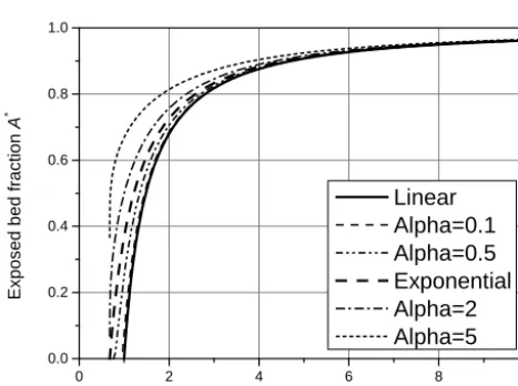
Figure 9. Variation of the exposed bed fraction as a function of transport capacity, assuming that particle speed scales with transport capacity to the power of one-third.

Using the exponential cover model (Eq. 8), we obtain

1 A∗_(1−A∗₎

∂A∗ ∂t∗ =q

∗

t. (39)

Equation (39) is separable and can be integrated to obtain

ln A∗−ln 1−A∗=t∗q_t∗+C. (40)

LettingA∗(t∗=0)=A∗₀, whereA∗₀is the initial cover, the final equation is in the form of a sigmoidal-type function:

A∗= 1

1+ _1−A∗

0

A∗₀

e−t∗_q∗

t

. (41)

By making the parameters in the exponent on the right-hand side of Eq. (42) dimensional, we get

t∗q_t∗= t T

T LM0

qt=

t qt

LM0

, (42)

which allows a characteristic system timescaleTE to be

defined as

TE=

LM0

qt

. (43)

Since this timescale is dependent on the transport capac-ityqt, we can view it as a timescale associated with the

en-trainment of sediment from the bed (cf. Eq. 20) – hence the subscript “E” onTE. From Eq. (41), the exposed bed

frac-tion evolves in an asymptotic fashion towards equilibrium (Fig. 11). We can expect that there are other characteristic timescales for the system, for example associated with sedi-ment deposition or downstream sedisedi-ment evacuation.

We can make some further progress and define a more gen-eral system timescale by performing a perturbation analysis (Appendix A1). For small perturbations in eitherq_s∗ orq_t∗, we obtain an exponential term describing the transient evo-lution, which allows the definition of a system timescaleTS

expn−q_t∗−1−e−qs∗U∗

q∗

s

t∗o=e− t

TS_{. (44)}

Here, exp denotes the natural exponential function. The characteristic system timescale can then be written as

TS=

LM0

qt

1−1−e−q∗ sU∗

_q s

qt =

LM0

qt

eMs∗_{. (45)}

Note that forq_s∗=0, Eq. (45) reduces to Eq. (43), as would be expected. SinceM∗

s is directly related to steady-state bed

exposureA∗_{, we can rewrite the equation, for example by}

assuming the exponential cover function (Eq. 8), as

TS=

LM0

qtA∗

. (46)

Since bed cover is more easily measurable than the mass on the bed, Eq. (46) can help to estimate system timescales in the field. Further,A∗_{varies between 0 and 1, which allows}

0 2 4 6 8 10 0.0

0.2 0.4 0.6 0.8 1.0

0 2 4 6 8 10

0.0 0.2 0.4 0.6 0.8 1.0

R

el

at

iv

e t

rans

por

t r

at

e _{Sediment input} Sediment output

E

xpos

ed bed f

rac

tion,

di

m

ens

ionl

es

s m

as

s

Dimensionless time t* Exposed bed fraction

Mobile mass Stationary mass

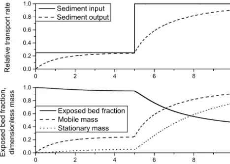
Figure 10.Temporal evolution of cover for the simple case of a control box with sediment through-flux, based on Eqs. (3), (22), (23), and (24). Relative sediment supply (supply normalized by transport capacity) was specified to 0.25 and increased to 1 at

t∗=5. The response of sediment output, mobile and stationary sed-iment mass, and the exposed bed fraction was calculated. Here, we used the exponential function forP(Eq. 8) andM₀∗=U∗=1. The initial values wereA∗=1 andM_m∗ =M_s∗=0.

To illustrate these additional dependencies, we have used numerical solutions of Eqs. (3), (22), (23), and (24) to calcu-late the time needed to reach 99.9 % of total adjustment after a step change in transport stage (chosen due to the asymptotic behaviour of the system), analysed across a plausible range of particle speeds U (Fig. 12). Response time decreases as particle speed increases. This reflects elevated downstream evacuation for higher particles speeds, resulting in a smaller mobile particle mass and thus higher entrainment and lower deposition rates. Response time also increases with increas-ing relative sediment supplyQ∗_s. As the runs start with zero sediment cover and the extent of cover increases withQ∗_s, at higherQ∗_sthe adjusted cover takes longer to develop.

3.3.2 Phase shift and gain in response to a cyclic perturbation

The perturbation analysis (Appendix A) gives some insight into the response of cover to cyclic sinusoidal perturbations. Let sediment supply be perturbed in a cyclic way described by an equation of the form

q_s∗=q∗

s +δq

∗

s =qs∗+d sin

₂ π t p

. (47)

Here, the overbar denotes the temporal average,δq_s∗is the time-dependent perturbation,dis the amplitude of the pertur-bation, andpits period. A similar perturbation can be applied to the transport capacity (see Appendix A). The reaction of the stationary mass and therefore cover can then also be

de-0 2 4 6 8 10

0.0 0.2 0.4 0.6 0.8 1.0

E

xpos

ed bed f

rac

tion

A

*

Dimensionless time t*

Figure 11.Evolution of the exposed bed fraction (removal of sed-iment cover) over time starting with different initial values of bed exposure, for the special case of no sediment supply; i.e.q_s∗=0 (Eq. 41) andq_t∗=1.

scribed by sinusoidal function of the form (Appendix A)

δM_s∗=Gsin _{2π t}

p +ϕ

. (48)

Here,δM_s∗ is the perturbation of the stationary sediment mass around the temporal average,Gis known as the gain, describing the amplitude response, andϕis the phase shift. If the gain is large, stationary mass reacts strongly to the pertur-bation; if it is small, the forcing does not leave a signal. The phase shift is negative if the response lags behind the forcing and positive if it leads. The phase shift can be written as

ϕ=tan−1

−2πTS p

. (49)

The gain can be written as

G= p

TS

Kd r

p TS

2 +4π2

. (50)

Here,d is the amplitude of the perturbation, andK is a function of the time-averaged values of qs, qt, and U and

differs for perturbations in transport capacity and sediment supply (see Appendix A). Thus, the system behaviour can be interpreted as a function of the ratio of the period of pertur-bationp and the system timescaleTs. The periodpis large

if the forcing parameter, i.e. discharge or sediment supply, varies slowly and small when it varies quickly. According to Eq. (49), the phase shift is equal to−π/2 for low values of p/Ts (quickly varying forcing parameter), implying a

sub-stantial lag in the adjustment of cover. The phase shift tends to 0 asp/Ts tends to infinity (Fig. 13). The gain varies

ap-proximately linearly withp/Tsfor smallp/Ts(quickly

0.0 0.2 0.4 0.6 0.8 1.0 1.2 0

10 20 30 40 50 60 70 80 90 100

0.0 0.2 0.4 0.6 0.8 1.0

0 10 20 30 40 50 60 70 80 90 100

(b)

99

.9

%

re

sp

on

se

ti

m

e

Relative sediment supply Q* s

Particle speed 0.05 m s–1

0.075 0.1 0.25 0.5 0.75 1

(a)

Particle speed U* _{/ m s–1}

Relative sediment supply

0.2 0.4 0.6 0.8 1 1.2 m s–1

m s–1

m s–1

m s–1

m s–1

m s–1

Figure 12.Dimensionless time to reach 99.9 % of the total adjustment in the exposed area as a function of(a)transport stage and(b)particle speed. All simulation were started withA∗=1 andM_m∗=M_s∗=0.

0 2 4 6 8 10 12 14 16 18 20

-1.5 -1.0 -0.5 0.0 0.5 1.0

Gain

G

ai

n,

p

ha

se

s

hi

ft

p/T_S

Phase shift

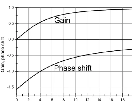
Figure 13.Phase shift (Eq. 49) and gain (Eq. 50) as a function of the ratio of the period of perturbationp and the system timescale

Ts. For the calculation, the constant factor in the gain (Kd) was set equal to 1.

a value ofKdfor largep/Ts(slowly varying forcing

param-eter) (Eq. 50). Thus, if the forcing parameter varies slowly, cover adjustment keeps up at all times.

3.3.3 A flood at the Erlenbach

To illustrate the magnitude of the timescales using real data, we use a flood data set from the Erlenbach, a sediment trans-port observatory in the Swiss Prealps (e.g. Beer et al., 2015). There, near a discharge gauge, bedload transport rates are measured at 1 min resolution using the Swiss Plate Geophone System, a highly developed and fully calibrated surrogate bedload measuring system (e.g. Rickenmann et al., 2012; Wyss et al., 2016). We use data from a flood on 20 June 2007 (Turowski et al., 2009) with the highest peak discharge that has so far been observed at the Erlenbach. The meteorolog-ical conditions that triggered this flood and its geomorphic

effects have been described in detail elsewhere (Molnar et al., 2010; Turowski et al., 2009, 2013). The Erlenbach does not have a bedrock bed in the sense that bedrock is exposed in the channel bed; however, the data provide a realistic nat-ural time series of discharge and bedload transport over the course of a single event. Rather than predicting bed cover evolution for a natural system, for which we do not currently have data for validation, we use the Erlenbach data to illus-trate possible cover behaviour during a fictitious event with different initial sediment cover extents, using natural data to provide realistic boundary conditions.

Using a median grain size of 80 mm, a sediment density of 2650 kg m−3, and a reach length of 50 m, we obtained M0=128 kg m−2. We calculated transport capacity using

the equation of Fernandez Luque and van Beek (1976). How-ever, it is known that this and similar equations strongly over-estimate measured transport rates in streams such as the Er-lenbach (e.g. Nitsche et al., 2011). Consequently, we rescaled by setting the ratio of bedload supply to capacity to 1 at the highest discharge. The exposed fraction was then calculated iteratively assumingP =A∗(i.e. the exponential cover for-mulation, Eq. 8). In a real flood event, water discharge and sediment supply obviously do not follow a small cyclic per-turbation (Fig. 13). But we can tentatively relate the obser-vations to the theory by assuming that at each time step, the change in sediment supply can be represented by the com-mencement of a sinusoidal perturbation with varying period. To estimate the effective period p, one needs to take the derivatives of Eq. (47).

dq_s∗ dt =

dδq_s∗ dt =

2π d

p cos

_{2π t}

p

(51)

Settingt=0 for the time of interest, we can relate pto the local gradient in bedload supply, which can be measured from the data.

2π d

p =

1q_s∗

Assuming that all change in the response time is due to changes in the period (i.e. assuming a constant amplitude, d=1), we can obtain a conservative estimate of the range over whichpvaries over the course of an event.

p=2π 1t 1q∗

s

(53)

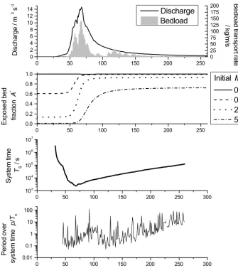
In the exemplary event, the evolution and final value of bed cover depends strongly on its initial value (Fig. 14), indicat-ing that the adjustment is incomplete. The system timescale is generally larger than 1000 s and is inversely related to dis-charge via the dependence on transport capacity. The p/Ts

ratio varies around 1, with low values at the beginning of the flood and large values in the waning hydrograph. Both the high values of the system timescale and the smooth evolution of bed cover over the course of the flood imply that cover development cannot keep up with the variation in the forc-ing characteristics. This dynamic adjustment of cover, which can lag forcing processes, may thus play an important role in the dynamics of bedrock channels and probably needs to be taken into account in modelling.

4 Discussion

4.1 Model formulation

In principle, the framework for the cover effect presented here allows the formulation of a general model for bedrock channel morphodynamics without the restrictions of previ-ous models (e.g. Nelson and Seminara, 2011; Zhang et al., 2015). To achieve this, the dependency ofP on various con-trol parameters needs to be specified. In general, P should be controlled by local topography, grain size and shape, hy-draulic forcing, and the amount of sediment already resid-ing on the bed. Furthermore, the shape of the P function should also be affected by feedbacks between these prop-erties, such as the development of sediment cover altering the local roughness and hence altering hydraulics and local transport capacity (Inoue et al., 2014; Johnson, 2014). In the treatment presented here, we have explicitly accounted only for the impact of the amount of sediment already residing on the bed. However, all of the mentioned effects can be in-cluded implicitly by an appropriate choice of P. The exact relationships between, say, bed topography andP need to be mapped out experimentally (e.g. Inoue et al., 2014), with the-oretical approaches also providing some direction (cf. John-son, 2014; Zhang et al., 2015). Currently available experi-mental results (Chatanantavet and Parker, 2008; Finnegan et al., 2007; Hodge and Hoey, 2016; Inoue et al., 2014; Johnson and Whipple, 2007) cover only a small range of the possible parameter space, and, in general, not all necessary parame-ters to constrain P were reported. Specifically the station-ary mass of sediment residing on the bed is usually not re-ported and can be difficult to determine experimentally but is necessary to determineP. Nevertheless, depending on the

choice ofP, our model can yield a wide range of cover func-tions that encompasses reported funcfunc-tions both from numer-ical modelling (e.g. Aubert et al., 2016; Hodge and Hoey, 2012; Johnson, 2014) and experiments (Chatanantavet and Parker, 2008; Inoue et al., 2014; Sklar and Dietrich, 2001) (see Figs. 4 and 5).

The dynamic model put forward here is a minimum first-order formulation, and there are some obvious future alter-ations. We only take account of the static cover effect caused by immobile sediment on the bed. The dynamic cover effect, which arises when moving grains interact at high sediment concentration and thus reduce the number of impacts on the bed (Turowski et al., 2007), could in principle be included in the formulation but would necessitate a second probability function specifically to describe this dynamic cover. It would also be possible to use differentP functions for entrainment and deposition, thus introducing hysteresis into cover devel-opment. Such hysteresis has been observed in experiments in which the equilibrium sediment cover was a function of the initial extent of sediment cover (Chatanantavet and Parker, 2008; Hodge and Hoey, 2012). Whether such alterations are necessary is best established with targeted laboratory experi-ments.

4.2 Comparison to previous modelling frameworks

We will briefly outline in this section the main differences to previous formulations of cover dynamics in bedrock chan-nels. Thus, the novel aspects of our formulation and the re-spective advantages and disadvantages will become clear.

Aubert et al. (2015) coupled the movement of spherical particles to the simulation of a turbulent fluid and investi-gated how cover depends on transport capacity and supply. Similar to what is predicted by our analytical formulation, they found a range of cover function for various model set-ups, including linear and convex-up relationships (compare the results in Fig. 6 to their Fig. 15). Aubert et al. (2015) pre-sented the most detailed physical simulations of bed cover formation so far, and the correspondence between the pre-dictions is encouraging.

-1

Figure 14.Calculated evolution of cover during the largest event observed at the Erlenbach on 20 June 2007 (Turowski et al., 2009). Bedload transport rates were measured with the Swiss Plate geophone sensors calibrated with direct bedload samples (Rickenmann et al., 2012). The final fraction of exposed bedrock is strongly dependent on its initial value.

can cover an entire grid node (cf. Fig. 1). Although different in various details, Inoue et al. (2016) have used essentially the same approach as Nelson and Seminar (2011, 2012) to link bedload concentration, transport, and bed cover. Both of these models allow the 2-D modelling of bedrock channel morphology. Although we have not fully developed such a model in the present paper, our model framework could eas-ily be extended to 2-D problems.

Inoue et al. (2014) formulated a 1-D model for cover dy-namics and bedrock erosion. There, they distinguish between stationary and mobile sediment using an Exner equation to capture sediment mass conservation. The degree of bed cover is related to transport rates and sediment mass via a satura-tion volume, which is related to our characteristic massM₀∗ (see Sect. 3.2). A key difference between Inoue et al.’s (2014) model and the ones presented here lies in the sediment mass conservation equations (Eqs. 13 and 14), in which we

explic-itly take account of both entrainment and deposition. In addi-tion, with the functionP, describing the relationship between deposited mass and degree of cover, we provide a more flexi-ble framework for complex simulations where the bed needs to be discretized (e.g. 2-D models or reach-scale formula-tions).

on roughness, and thus it allows a more general treatment of the problem of bed cover.

In this paper, we focused on the dynamics of bed cover rather than on the modelling of the dynamics of entire chan-nels. The probabilistic formulation using the parameter P provides a flexible framework to connect the sediment mass residing on the bed with the exposed bedrock fraction. This particular element has not been treated in any of the previous models and could be easily implemented in other approaches dealing with sediment fluxes along and across the stream and the interaction with erosion and, over long timescales, chan-nel morphology. However, it is as yet unclear how flow hy-draulics, sediment properties, and other conditions affectP, and this should be investigated in targeted laboratory experi-ments.

4.3 Further implications

Based on field data interpretation, Phillips and Jerol-mack (2016) argued that bedrock rivers adjust such that, sim-ilar to alluvial channels, medium-sized floods are most ef-fective in transporting sediment and that channel geometry therefore can quickly adjust their transport capacity to the applied load and therefore achieve grade (cf. Mackin, 1948). They conclude that bedrock channels can adjust their mor-phologic parameters (channel width and shape) quickly in response to changing boundary conditions. In contrast, our model suggests that instead bed cover can be adjusted to achieve grade. In steady state, time derivatives need to be equal to 0. Thus, entrainment equals deposition (Eq. 14), implying that the downstream gradient in sediment trans-port rate is equal to 0 (Eq. 13). When sediment supply or transport capacity change, the exposed bedrock fraction can adjust to achieve a new steady state, and a change in the channel geometry is unnecessary. These changes in sedi-ment cover can occur far more rapidly than changes in width and cross-sectional shape (compare to Eq. 46). Whether a steady state is achieved depends on the relative magnitude of the timescales of perturbation and cover adjustment (see Sect. 3). Our results imply that bedrock channels have two distinct timescales to adjust to changing boundary conditions to achieve grade. Over short times, bed cover is adjusted. This can occur rapidly. Over long timescales, channel width, cross-sectional shape, and slope are adjusted.

5 Conclusions

The probabilistic view put forward in this paper offers a framework into which diverse data on bed cover, whether ob-tained from field studies, laboratory experiments, or numer-ical modelling, can be easily converted to be meaningfully compared. The conversion requires knowledge of the mass of sediment on the bed and the evolution of exposed fraction of the bed. Within the framework, individual data sets can be compared to the exponential benchmark and linear limit cases, enabling physical interpretation. Furthermore, the for-mulation allows the general dynamic sub-grid modelling of bed cover. Depending on the choice ofP, the model yields a wide range of possible cover functions. Which of these func-tions are appropriate for natural rivers and how they vary with factors including topography needs to mapped out ex-perimentally.

It needs to be noted here that the precise formulation of the entrainment and deposition functions also affects steady-state cover relations. When calibrating P on data, it can-not always be decided whether a specific deviation from the benchmark case results from varying entrainment and depo-sition processes or from changes in the probability function driven for example by variations in roughness. For the pre-diction of the steady-state cover relations and for the com-parison of data sets, this should not matter, but the dynamic evolution of cover could be strongly affected.

The system timescale for cover adjustment is inversely re-lated to transport capacity. This timescale can be long and in many realistic situations, cover cannot instantaneously adjust to changes in the forcing conditions. Thus, dynamic cover ad-justment needs to be taken into account when modelling the long-term evolution of bedrock channels.

Our model formulation implies that bedrock channels ad-just bed cover to achieve grade. Therefore, bedrock channel evolution is driven by two optimization principles. On short timescales, bed cover adjusts to match the sediment output of a reach to its input. Over long timescales, width and slope of the channel evolve to match long-term incision rate to tec-tonic uplift or base-level lowering rates.

Appendix A: Perturbation analysis

Here, we derive the effect of a small sinusoidal perturba-tion of the driving variables, namely sediment supplyq_s∗and transport capacityq_t∗, on cover development. The perturba-tion of the driving variables can be written as

q_s∗=q∗

s +δq

∗

s, (A1)

q_t∗=q_t∗+δq_t∗. (A2)

Here, the bar denotes the average of the quantity at steady state, whileδq_s∗ andδq_t∗denote the small perturbation. The exposed area can be similarly written as

A∗=A∗_+δA∗

. (A3)

Steady-state cover is directly related to the mass on the bed M_s∗by Eq. (3), which, as long asP is independent of time, we can rewrite as

dA∗ dt = −P

dM_s∗

dt . (A4)

Substituting Eq. (A3) and a similar equation forM_s∗,

M_s∗=M∗

s +δM

∗

s, (A5)

we obtain

dδA∗ dt = −P

dδM_s∗

dt . (A6)

Here, the averaged terms drop out as they are independent of time. IfP and the steady-state solution forA∗are known, a direct relationship betweenA∗andM_s∗can be derived. For example, for the exponential cover model (Eq. 8), substitut-ing Eqs. (A3) and (A5), we find

A∗_+δA∗ _=e−M∗

s−δMs∗_=e−Ms∗_e−δMs∗_=A∗_e−δMs∗ _(A7)

≈A∗ _1−δM∗

s

.

Here, since theδvariables are small, we approximated the exponential term using a Taylor expansion to first order. We obtain perturbation of sediment supply

δA∗= −A∗_δM∗

s. (A8)

It is therefore sufficient to derive the perturbation solution for M_s∗, the time evolution of which is given by Eq. (22). EliminatingM_m∗ using Eq. (24), we obtain

∂M_s∗ ∂t∗ =

1−e−q∗s/U∗

q_s∗−1−e−M∗s

q_t∗. (A9)

A1 Perturbation of sediment supply

First, let us look at a perturbation of sediment supply q_s∗, while other parameters are held constant. Substituting

Eqs. (A1) and (A5) into Eq. (A9), we obtain

∂δM_s∗ ∂t∗ =

1−e−qs∗+δqs∗

/U∗ q∗

s +δq

∗

s

(A10)

−1−e−Ms∗−δMs∗

q_t∗.

Again, since theδvariables are small, we can replace the relevant exponentials with a Taylor expansion to first order:

e−δqs∗/U∗_≈1−δq

∗

s

U∗. (A11)

A similar approximation applies for the exponential inM_s∗. Substituting Eq. (A11) into Eq. (A10), expanding the multi-plicative terms, dropping terms of second order in theδ vari-ables and rearranging, we get

∂δM_s∗ ∂t∗ =δq

∗

s

1−e−qs∗U∗+ q

∗

s

U∗e −q∗

s/U∗

(A12)

−δM_s∗

q_t∗−

1−e−qs∗/U∗

q∗

s

.

The perturbation is assumed to be sinusoidal

δq_s∗=dsin _{2π t}

p

. (A13)

Here,pis the period of the perturbation andd is its am-plitude. Note that, to be consistent with the assumptions pre-viously made,d needs to be small in comparison with the average sediment supply. Substituting, Eq. (A12) can be in-tegrated to obtain the solution

δM_s∗=Gq∗ ssin

_{2π t}

P +ϕq ∗ s

+C (A14)

exp

−q_t∗−1−e−qs∗/U∗ q∗ s t T ,

whereCis a constant of integration. The gain is given by

Gq∗ s =

p T

1−e−qs∗/U∗+qs∗

U∗e−q ∗ s/U∗

d

r

q_t∗−

1−e−qs∗/U∗ q∗ s 2 p T 2 +4π2

(A15)

and the phase shift by

ϕq∗ s =tan

−1  − 2π p T

q_t∗−1−e−qs∗/U∗

q∗

s



. (A16)

A2 Perturbation of transport capacity

problem, we expand the exponential term featuringU∗(δq_t∗) in Eq. (A9) using a Taylor series expansion aroundδq_t∗=0.

exp (

− q

∗

s

U∗ _δq∗

t ) (A17) ≈ exp ( − q ∗ s

U∗ _δq∗

t =0

)

"

1− q

∗

s

U∗2

δq_t∗=0 ∂U∗

∂δq_t∗ δq ∗

t =0

δq_t∗

#

BothU∗and its derivative are constants when evaluated at δq_t∗=0. We can thus write

exp −q ∗ s U∗ =exp −q ∗ s U∗ " 1− q

∗

s

U∗2

_∂U∗

∂δq_t∗

δq_t∗ #

=1−C0δqt∗

eqs∗/U∗_{. (A18)}

Here,C0is a constant. Proceeding as before by

substitut-ing Eqs. (A2), (A8), and (A17) into (A9), expandsubstitut-ing expo-nential terms containingδ variables, dropping terms of sec-ond order in theδvariables, and rearranging, we obtain

∂δM_s∗

∂t∗ = (A19)

Bq_s∗e−qs∗/U∗+e−Ms∗−1δq_t∗−δM_s∗q_t∗e−Ms∗_.

A sinusoidal perturbation of the form

δq_t∗=dsin _{2π t}

p

(A20)

yields the solution

δM_s∗ =Gq∗ t sin

_{2π t}

P +ϕqt∗

(A21)

+Cexp

−

q_t∗−

1−e−q∗s/U∗

q_s∗ t p − q_t∗−

1−e−qs∗/U∗

q_s∗ t T

,

with

Gq_t∗=

p T

qs∗2

U∗2

∂U∗

∂δq∗ t

e−qs∗/U∗−1−e−q∗s/U∗ _q∗ s q∗ t d s

q_t∗2 p_T2

1− 1−e−qs∗/U∗q ∗ s

q∗ t

2 +4π2

(A22)

and

ϕ=tan−1  − 2π p T

q_t∗−1−e−q∗ s/U∗

q∗

s



. (A23)

A3 Summary

Using the system timescaleTS, the phase shift and gain can

be generally rewritten as

ϕ=tan−1

−2πTS p

, (A24)

G= p

TS Kd r _p TS 2

+4π2

. (A25)

Here,K differs for perturbations in sediment supply and transport capacity, given by the equations

Kq∗ s =1−e

−q∗ s/U∗₊ q

∗

s

U∗e −q∗

s/U∗_{, (A26)}

Kq∗ t =

q_s∗2

U∗2

_∂U∗

∂δq_t∗

e−qs∗/U∗−1−e−qs∗/U∗ q∗

s

Appendix B: Notation

Overbars denote time-averaged quantities. a Shape parameter in the regularized

incomplete Beta function

A∗ Fraction of exposed (uncovered) bed area A∗_c Fraction of covered bed area

b Shape parameter in the regularized incomplete Beta function

B Regularized incomplete Beta function C Constant of integration

C0 Constant (m2s kg−1)

d Amplitude of perturbation (kg m−2s)

D Sediment deposition rate per bed area (kg m−2s) Dtot Sediment deposition rate (kg s−1)

D∗ Dimensionless sediment deposition rate D50 Median grain size (m)

e Base of the natural logarithm

E Sediment entrainment rate per bed area (kg m−2s) Etot Sediment entrainment rate (kg s−1)

E∗ Dimensionless sediment entrainment rate Emax Maximal possible dimensionless

sediment entrainment rate

g Acceleration due to gravity (m s−2) G Gain (kg m−2_s)

I Non-dimensional incision rate

k Probability of sediment deposition on uncovered parts of the bed, linear implementation

K Parameter in the gain equation L Characteristic length scale (m)

M0 Minimum mass per area necessary to cover

the bed (kg m−2)

M₀∗ Dimensionless characteristic sediment mass Mm Mobile sediment mass (kg m−2)

M_m∗ Dimensionless mobile sediment mass Ms Stationary sediment mass (kg m−2)

M∗

s Dimensionless stationary sediment mass

p Period of perturbation (s)

pc Probability of entrainment, CA model, blocked grains

pi Probability of entrainment, CA model, free grains

P Probability of sediment deposition on uncovered parts of the bed

qs Mass sediment transport rate per unit width (kg ms−1)

q_s∗ Dimensionless sediment transport rate qt Mass sediment transport capacity

per unit width (kg ms−1) q_t∗ Dimensionless transport capacity

Q∗_s Relative sediment supply; sediment transport rate over transport capacity

Qt Mass sediment transport capacity (kg s−1)

t Time variable (s) t∗ Dimensionless time T Characteristic timescale (s)

TE Characteristic timescale for

sediment entrainment (s)

TS Characteristic system timescale (s)

U Sediment speed (m s−1) U∗ Dimensionless sediment speed

x Dimensional streamwise spatial coordinate (m) x∗ Dimensionless streamwise spatial coordinate y Dummy variable

α Exponent

γ Fraction of pore space in the sediment δ Denotes time-varying component 1in Sediment supply rate from

upstream direction (kg s−1)

1out Transport rate of sediment leaving in the downstream direction (kg s−1) 1Mm Change in mobile sediment mass (kg)

1t Change in time (s) θ Shields stress θc Critical Shields stress

ρ Density of water (kg m−3) ρs Density of sediment (kg m−3)

τ Bed shear stress (N m−2)

τc Critical bed shear stress at the onset of