www.nonlin-processes-geophys.net/18/697/2011/ doi:10.5194/npg-18-697-2011
© Author(s) 2011. CC Attribution 3.0 License.
Nonlinear Processes
in Geophysics
Dynamical changes of the polar cap potential structure:
an information theory approach
I. Coco, G. Consolini, E. Amata, M. F. Marcucci, and D. Ambrosino
INAF-Istituto di Fisica dello Spazio Interplanetario, Via Fosso del Cavaliere, 100, 00133 Roma, Italy
Received: 28 February 2011 – Revised: 3 October 2011 – Accepted: 5 October 2011 – Published: 17 October 2011
Abstract. Some features, such as vortex structures often
ob-served through a wide spread of spatial scales, suggest that ionospheric convection is turbulent and complex in nature. Here, applying concepts from information theory and com-plex system physics, we firstly evaluate a pseudo Shannon entropy,H, associated with the polar cap potential obtained from the Super Dual Auroral Radar Network (SuperDARN) and, then, estimate the degree of disorder and the degree of complexity of ionospheric convection under different Inter-planetary Magnetic Field (IMF) conditions. The aforemen-tioned quantities are computed starting from time series of the coefficients of the 4th order spherical harmonics expan-sion of the polar cap potential for three periods, characterised by: (i) steady IMFBz>0, (ii) steady IMFBz<0 and (iii) a double rotation from negative to positive and then positive to negativeBz. A neat dynamical topological transition is ob-served when the IMFBzturns from negative to positive and vice versa, pointing toward the possible occurrence of an or-der/disorder phase transition, which is the counterpart of the large scale convection rearrangement and of the increase of the global coherence. This result has been confirmed by ap-plying the same analysis to a larger data base of about twenty days of SuperDARN data, allowing to investigate the role of IMFBytoo.
1 Introduction
High-latitude ionospheric convection is the result of direct coupling between the solar wind and the Earth’s magneto-sphere. The magnetospheric electric fields map down in the ionosphere giving rise to a motion of ions and electrons in the E×B direction: this results in a multi-cell pattern in
Correspondence to: I. Coco
the polar cap that is a “mirror” on a reduced space scale of the magnetospheric plasma motion. It is now well accepted that the most important parameter, which drives the dynam-ical processes in the magnetosphere-ionosphere system and the ionospheric convection pattern configuration, is the In-terplanetary Magnetic Field (IMF), whose orientation with respect to the Earth’s magnetic field is crucial for the amount of energy, momentum and plasma particles that can penetrate the magnetospheric cavity. When a quasi steady IMFBz<0 component is present (southward IMFBz), reconnection is thought to take place at the subsolar magnetopause, creating open field lines which are dragged towards the tail, where they reconnect again, pushing plasma back to the dayside magnetosphere along the flanks: the ionospheric convection is organised in a two-cell pattern, where plasma is flowing antisunward at high latitudes in the polar cap, and sunward at lower latitudes (Dungey convection cycle: e.g. Dungey, 1961). When IMF is dominated by a Bz>0 component (northward IMFBz), reconnection is favoured tailward of the polar cusps: now the open field lines are pushed sunward by the magnetic tension, and again a double cell pattern should appear in the polar caps, but in this case plasma flows sun-ward at very high latitudes and antisunsun-ward at lower latitudes (e.g. Burke et al., 1979; Huang et al., 2000). Reconnection in the tail can always occur due to the substorm cycle or unbal-anced reconnection processes in the far tail, giving rise to one or more convection cells in the nightside even for northward IMFBz; moreover, viscous processes at the magnetopause can produce elongated convection cells in the dusk and dawn ionosphere, that can be more evident when the Dungey con-vection cycle for southward IMFBzis not established (e.g. Axford and Hines, 1961; Cowley and Lockwood, 1992). In summary, the ionospheric convection for northward IMFBz is far less homogeneous than in the opposite case, showing the emergence of more than two convection cells due to sev-eral different competing mechanisms. The scheme is further complicated by the IMFBy component, which acts on the
symmetry of the convection patterns, rotating the cell sys-tem towards dawn or dusk according to the sign ofBy; in the limit of|By| |Bz|usually only one big convection cell is observed (e.g. Reiff and Burch, 1985; Gosling et al., 1990; Ruohoniemi and Greenwald, 1996, 2005).
On the other hand, evidences exist that the Earth’s mag-netosphere/ionosphere can be viewed as a physical system operating in a non-equilibrium dynamical state and display-ing dynamical complexity (e.g. Sharma and Kaw, 2005; Con-solini et al., 2008). Following Chang et al. (2006), dynam-ical complexity can be defined as “a phenomenon exhibited by a nonlinear interacting dynamical system within which multitudes of different sizes of large scale coherent struc-tures are formed, resulting in a global nonlinear stochastic behavior for the dynamical systems, which is vastly different from what could be surmised from the original dynamical equations”. In other words, complexity often shows up as the tendency of a non equilibrium system to display a cer-tain degree of spatio-temporally coherent features resulting from the competition of different basic spatial patterns play-ing the role of interactplay-ing subunits. It is important to remark that complexity requires the occurrence of nonlinearities and the intertwining of order and disorder (Nicolis and Nicolis, 2007) and that it is generally related to the emergence of self-organisation in open systems (Klimontovich, 1991, 1996).
In the last two decades, the evidence of large scale co-herence and multiscale nature of magnetospheric dynamics was clearly recognised in different ways, analysing both the low-dymensional behaviour of the large scale dynamics and the turbulent and critical nature of the small scale processes (e.g. Chang, 1992; Consolini et al., 1996; Klimas et al., 1996; Sharma and Kaw, 2005). In particular, the emergence of large scale coherence during magnetic substorms was inter-preted and modelled in terms of first-order phase transitions in out-of-equilibrium dynamical systems (Sitnov et al., 2000, 2001). The increase of coherence during magnetospheric disturbed periods is the signature of the emergence of long-range space-time correlation, and, to some extent, of large scale self-organisation.
The Super Dual Auroral Radar Network (SuperDARN, Greenwald et al., 1995; Chisham et al., 2007) is nowadays one of the most important instruments to reconstruct and monitor the high-latitude ionospheric convection. The Su-perDARN radars measure the Doppler shift of field-aligned density irregularities in the ionosphere which drift follow-ing the motion of the ambient plasma. The line of sight ve-locities of each radar are combined together using a tech-nique described in Ruohoniemi and Baker (1998), allow-ing to reconstruct the isocontours of the Polar Cap Poten-tial (PCP), which is closely related to the energy transfer from the solar wind to the magnetosphere and the ionosphere systems. A number of studies have now demonstrated that the maximum variations of the PCP on the dayside and on the nightside are equivalent to the reconnection rates, i.e. the rate of transfer of magnetic flux across unit length of
the separatrix between unreconnected and reconnected field lines (e.g. Chisham et al., 2008, and references therein).
Recently, several authors studied ionospheric convection in the framework of complex systems, using SuperDARN data. Among others, Abel et al. (2009) found that turbu-lent features typical of the solar wind are present in the high-latitude ionosphere in regions where open field lines map, and that the degree of intermittency is controlled by the IMF clock angle, while Parkinson (2006, 2008) found a complex scaling of the convection velocity fluctuations in the F-region ionosphere.
In this paper we aim at extending the idea of global first order phase transition to the magnetosphere-ionosphere cou-pled system, by evidencing the emergence of coherence and self-organisation in the high-latitude ionosphere during the increase of magnetospheric convection. For that purpose, we will concentrate on large scale features of ionospheric con-vection, such as vortices and cell-like convection patterns, whose configuration is modulated by the IMF, and will use concepts taken from information theory applied to the polar cap potential, in order to build up a measure of complexity in the way already followed by Shiner et al. (1999) and Con-solini et al. (2009). In particular, we aim at quantifying the spatial complexity of the polar cap potential and its depen-dence on the orientation of the IMF.
The paper is structured as follows: in Sect. 2, in the frame-work of information theory and complexity, we will define a pseudo Shannon entropy,H, the time dependent disorder degree, 1(t ), and the Second Order Complexity Measure, 011; in Sect. 3 the Ruohoniemi and Baker (1998) technique for obtaining the polar cap potential will be described in some more detail, and the application of the information the-ory concepts to the SuperDARN data will be introduced; in Sect. 4 we will first show the results for a couple of case stud-ies where the IMF is steadily southward/northward directed, and a case study where IMFBz is varying throughout the event (Sect. 4.1), evidencing how ordered/disordered config-urations are concentrated in periods of southward/northward IMF and how complexity shows up in “intermediate” states; then, in Sect. 4.2, we will analyze a larger data base of about twenty days of SuperDARN data during February 2002, en-compassing all possible IMF configurations and investigat-ing the effect of IMFBy on the emergence of complexity. Conclusions are drawn in Sect. 5.
2 Shannon entropy and complexity: a brief introduction
As shown in several contexts, the investigation of complex dynamics may benefit from the application of concepts de-veloped in the framework of information theory (e.g. Haken, 2004; Nicolis and Nicolis, 2007). Indeed, the information theory methods, based on probability theory and statistics concepts, allow a different approach to the dynamics of
complex systems, characterised by a multitude of interact-ing scales, approach which is able to extract and charac-terise some common and universal features of complex sys-tems. For instance, Shannon entropy, mutual information and transfer entropy have been successfully applied to investi-gate the occurrence of phase transitions in several dynamical complex systems, ranging from the flocking model (Wicks et al., 2007), to physiology (Quian Quiroga et al., 2000), to the solar cycle (Sello, 2000, 2003; Consolini et al., 2009), to the evolution of the geomagnetic field (De Santis et al., 2004), to magnetospheric dynamics (Chen et al., 2008; De Michelis et al., 2011).
One of the major results of information theory surely stands on the concept of information entropy, originally in-troduced by Claude Shannon (Shannon, 1948) and for this reason also named Shannon entropy. This quantity is defined as follows:
SI= − N
X
i=1
pilog2(pi), (1)
wherepi is the probability of observing a certain state (con-figuration or value) over a set of N possible states (con-figurations or values). In the framework of signal analy-sis the Shannon entropy,SI, represents the average amount of code length needed to encode a randomly chosen value. However, it can be considered as a measure of the infor-mation/uncertainty content in a certain distribution of states (configurations or values). Furthermore, on the basis of the definition given in Eq. (1), the Shannon entropy,SI, takes its largest valueSImax=log2N in the case of equiprobable distributions (pi=1/N) and its smallest valueSImin=0 for δ−like distributions. The Shannon entropy,SI, also satisfies all the properties of additivity and convexity, required by a properly defined entropy.
Although the original concept of Shannon entropy was introduced to characterise the information content of a se-quence of discrete and independent random variables having Npossible outcomesxi(i=1,...,N) with associated proba-bilitiespi, in the course of the years the definition of Shan-non entropySI has been also extended to those situations in which the quantitiespi are not probabilities of outcomes but statistical and/or relative weights of an observable (e.g. Quian Quiroga et al., 2000; Sello, 2000; De Santis et al., 2004). For instance, Quian Quiroga et al. (2000) defined pi as the normalised spectral density at the frequency ωi, i.e. pi=S(ωi)/PiS(ωi), which is analogous to a relative weight.
The application of Shannon entropy to the case of statis-tical weights relies on the mathemastatis-tical definition of proba-bility in terms of a positive defined Lebesgue measureµ(A) normalised to 1. For instance, in the Feller’s book (Feller, 1970), page 22, we read: “Given a discrete sample space
E with sample pointsE1, E2, . . ., we shall assume that
with each point Ej there is associated a number, called
probability of Ej and denoted by P{Ej}. It is to be
non-negative and such that P{E1} +P{E2} +...=1.”
Further-more, the assumption of pi’s as relative statistical weights of spectral densities in different frequency domains is quite common also in the investigation of self-organisation in far-from-equilibrium open systems (e.g. Klimontovich, 1995).
In the following of this paper, we will replace thepi prob-abilities in Eq. (1) by the relative weights of given eigenfunc-tions of an observable,wi, so as to build an analogue of the Shannon entropy, that we call pseudo Shannon entropy,H. BecauseH attains its maximum value,Hmax=log2(N ), for a uniform distribution (i.e. the case ofwi =1/N, whereN is the number of eigenfunctions considered), the definition of the following normalised quantity turns to be helpful in comparing different configurations of a dynamical system:
1= H
Hmax= − 1 log2(N )
N
X
i=1
wilog2(wi), (2)
which can attain values in the interval[0,1].
Because the minimum and maximum values ofH corre-spond to the two extreme situations of monochromatic (sin-gle mode) spectra (δ−like distribution ofwi) and flat spec-tra (uniform distribution with equiprobablewi), the values 1=0 and 1=1 can be associated with maximum order and maximum disorder of the system described by the given eigenfunctions. The quantity 1was originally introduced by Landsberg (1978) (see also Landsberg, 1984) and pro-vides a measure of the degree of disorder. From definition of Eq. (2) it follows that a measure of order (degree of or-der) is=1−1. Because in the case of a nonequilibrium system a measure of the distance from equilibrium is pro-vided by the quantity S−Seq (Ebeling and Klimontovich, 1984; Klimontovich, 1995, 1996), whereS andSeq are the entropies of the nonequilibrium and of the equilibrium states respectively, and because in statistical thermodynamics the state of maximum entropy is the equilibrium one, it follows that=(Seq−S)/Seq really represents a measure of order in terms of normalised distance from equilibrium.
Several attempts have been made in the past in or-der to characterise the degree of complexity and/or self-organisation in non-equilibrium systems. Among the wide variety of definitions, one particularly simple and easy to compute was introduced by Landsberg and Shiner (1998) and Shiner et al. (1999). This complexity measure, 011, is defined as
011=1·=1(1−1)=(1−), (3) which is a special case of more general complexity mea-sures0αβ=1αβ. According to the above definition, the complexity measure011 implies that a non-vanishing level of complexity is possible only in nonequilibrium systems with some less than maximal order (Shiner et al., 1999). Al-though to a first reading one could conclude that all the re-quired information on the complex nature of the observed
phenomenon is contained in the degree of disorder 1 (or equivalently in the degree of order) this is not correct. In-deed, one way to define complexity is that it mainly arises in those situations where there is a certain competition be-tween order and disorder. This is the reason for defining as a measure of complexity the product of order and disorder, i.e. a quantity which is not a linear function of order or dis-order. In this framework, the measure of complexity011and the disorder measure1provide complementary information. We remark that according to the definition of011, the same degree of complexity can be found for situations in which the degree of disorder or that of order dominates. However, the emerging of complexity achieves a different meaning in the two situations. Thus, a better characterization of the complex nature of the system arises from the specification of its state in the{1,011}-space.
3 Data analysis methodology
SuperDARN radars work in “common” operating mode for most of the time, which means that they are synchronized over the whole polar cap, giving one- and two-minutes time series of the line-of-sight (l.o.s.) ionospheric convection ve-locity as a function of magnetic latitude and longitude. The l.o.s. velocity is just a component of the actual velocity vector in the direction along which the radar points during a given time interval. To reconstruct the whole velocity field over the polar cap, so that it matches as closely as possible the “true” ionospheric convection, all measurements in the radar reference frames are first averaged and median filtered over a common spatial grid of approximately 1◦×1◦Altitude Ad-justed Corrected Geomagnetic coordinates (AACGM, Baker and Wing, 1989). Successively, to fill the coverage gaps of the radar fields of view, a certain amount of model data is uniformely added up: these data come from empirical mod-els built over years of SuperDARN measurements and are chosen to represent the average convection patterns expected for the IMF configuration at the given ttime (Ruohoniemi and Greenwald, 1996, 2005). The technique by Ruohoniemi and Baker (1998) aims to reconstruct the isocontours of the PCP, 8, at timet, through a spherical harmonics expansion as fol-lows:
8(θ,ϕ;t )= <e{ ∞ X
l=0 l
X
m=0
clm(t )exp(imϕ)Plm(cos(θ ))}, (4)
whereθandϕare the AACGM colatitude and longitude,Plm are the Legendre polynomial functions, andclmare complex time-dependent coefficients. Writingclm(t )=Alm−iBlmin the Eq. (4) and calculating the real part, Eq. 4 can be simpli-fied as follows:
8(θ,ϕ;t )= ∞ X
l=0 l
X
m=0
(Almcos(mφ)+Blmsin(mφ))∗ (5) ∗Plm(cos(θ )).
Here, the expansion terms have been fully normalised, so that the quantity|clm|2=(A2lm+Blm2 )are representative of the variance (mean square value) associated with the compo-nent{l,m}(Lowes, 1966). Of course, in principlel varies from 0 up to∞in Eqs. (4) and (6), but in practice the ex-pansion is truncated to a finite order,L. The coefficients are evaluated through a least square fit of the function:
χ2= N
X
i=1 1 σi2
[V[i] ·kˆ[i] −Wi]2, (6)
whereWi andσi are the measured values of the velocity and their standard deviations in thei-th grid cell as defined above, while V[i]are the actual vector velocities to be calculated re-membering that V=(E×B)/B2in a quasi collisionless high altitude ionosphere (>300 km, where most of SuperDARN backscatter comes from), and E= −∇8, with E and B being the ionospheric electric field and the Earth’s magnetic field, respectively. The scalar product in Eq. (6), means that the vector V[i]has to be projected along the direction, ˆk, where Wihas been measured. It has been demonstrated that, even in the presence of quite wide spatial gaps in the data, if the data distribution is uniform through the pattern, the model data do not affect very much the final result, and the overall patterns are really dominated by the measured data (Shepherd and Ruohoniemi, 2000). The velocity vectors V[i]so obtained are always tangent to the equipotential contours. Now, fol-lowing what reported in Sect. 2 and moving from the expan-sion of Eq. (4), we introduce a discrete sample spaceϒ{l,m}, whose elements are the harmonic functionsϒl,m=exp(imφ) Plm(cos(θ )), and associate to each element of this space a time-dependent numberwl,m(t ), named relative weight and defined as follows:
wl,m(t )=
|cl,m(t )|2
P
j,k|cj,k(t )|2
, (7)
wherej,l∈ [0,L], beingLthe truncation order of the ex-pansion, and k,m∈ [0,L]. Such a quantity wl,m(t ) repre-sents the fraction of the variance (mean square value) of the field8(θ,φ;t )relative to the elementϒl,mat the timet, i.e. a measure of the relative relevance of the term ϒl,m at the timet. The spectrum of the relative weightswl,mis equiva-lent to a time-dependent normalised spectrum. Here we limit our analysis only to the investigation of thel spectrum, and instead of the relative weightswl,m(t )we consider:
-14 -12 -10 -8 -6 -4 -2 0 IMF B z (nT) 19.30
01/10/2003 20.00 20.30 21.00 21.30
Time (UT) 1.0 0.8 0.6 0.4 0.2 0.0 (t) IMF Bz (t) -03 -03 -09 -09 -09 -15 -15 -21 -27 03 03 09 09 15
01 Oct 2003 19:30:00 - 19:32:00 UT
0 m/s
1000 07 nT
(-00 min) +Y +Z 58 kV 00 MLT 06 12 MLT 18 -03 -03 -03 -03 -09 -09 -15 -15 -21 -21 -27 03 03 09 09
01 Oct 2003 20:30:00 - 20:32:00 UT
0 m/s
1000 09 nT
(-00 min) +Y +Z 50 kV 00 MLT 06 12 MLT 18 -03 -03 -03 -09 -09 -15 03 03 03 09 09 09 15 15 21
01 Oct 2003 21:28:00 - 21:30:00 UT
0 m/s
1000 12 nT
(-00 min) +Y +Z 50 kV 00 MLT 06 12 MLT 18
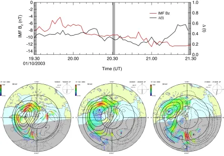
Fig. 1. Upper panel: IMFBz (red, axis on the left) as obtained by OMNI, and normalised disorder degree
Δ(t)(black, axis on the right), for the period 01/10/2003, 19:30 – 21:30 UT. Lower panel: three samples of
SuperDARN convection maps for the same period; the 2-minute scan intervals represented in the maps are shaded in the upper panel plot.
SuperDARN measurements and are chosen to represent the average convection patterns expected for
the IMF con
fi
guration at the time given (Ruohoniemi and Greenwald, 1996, 2005). The technique by
Ruohoniemi and Baker (1998) aims to reconstruct the isocontours of the PCP,
Φ
, at time
t
, through
a spherical harmonics expansion as follows:
Φ(
θ,ϕ
;
t
) =
e
{
∞
l=0 l m=0c
lm(
t
)exp(
imϕ
)
P
lm(cos(
θ
))
}
,
(4)
200
where
θ
and
ϕ
are the AACGM colatitude and longitude,
P
ml
are the Legendre polynomial functions,
and
c
lmare complex time-dependent coef
fi
cients. Writing
c
lm(
t
) =
A
lm−
iB
lmin the Eq. 4 and
calculating the real part, Eq. 4 can be simpli
fi
ed as follows:
Φ(
θ,ϕ
;
t
) =
∞ l=0 l m=0(
A
lmcos(
mφ
)+
B
lmsin(
mφ
))
∗
(5)
∗
P
lm(cos(
θ
))
.
205
Here, the expansion terms have been fully normalised, so that the quantity
|
c
lm|
2= (
A
2lm+
B
lm2)
are representative of the variance (mean square value) associated with the component
{
l,m
}
(Lowes,
7
Fig. 1. Upper panel: IMFBz(red, axis on the left) as obtained by OMNI, and normalised disorder degree1(t )(black, axis on the right), for
the period 01/10/2003, 19:30–21:30 UT. Lower panel: three samples of SuperDARN convection maps for the same period; the 2-min scan intervals represented in the maps are shaded in the upper panel plot.
wl(t )= l
X
m=0
wl,m(t )=
P
m|cl,m(t )|2
P
j,k|cj,k(t )|2
, (8)
wherewl(t )is representative of the total relative weight of harmonic functions of degreel. From here we can compute the time dependent disorder degree1(t ),
1(t )= − 1 log2(L+1)
L
X
l=0
wl(t )log2[wl(t )] (9)
and the corresponding time-dependent complexity measure 011(t ),
011(t )=1(t )[1−1(t )], (10) following the definitions given in Sect. 2. According to the given eigenfunction series expansion, the meaning of the quantities1and011as measures of disorder and complexity has to be related to the formation of single/multi scale spatial fluctuations. If1=0, we are in the presence of a monochro-matic spectrum, so that the spatial fluctuations are mainly characterised by a limited set of scales (in the extreme case, by one scale only); conversely,1=1 corresponds to a flat
spectrum which is associated to multiscale fluctuations. In this framework, complexity shows up in intermediate condi-tions, i.e. when there is a certain number of fluctuation scales interacting and evolving in time.
4 Results and discussion
We have applied the formalism described in the previous Sections to time series of PCP coefficients as obtained from Eqs. (4) and (6) through the Ruohoniemi and Baker (1998) technique. The expansion of the PCP has been limited to the fourth order, as we have checked that the results do not change substantially if we use higher order expansions.
4.1 Case studies for different IMF orientations
We first consider two two-hour intervals of SuperDARN data in the Northern Hemisphere, characterised by almost steady conditions of the IMF and good overall coverage.
In Figure 1, upper panel, the IMFBz(red curve) is shown for the 19:30–21:30 UT period on 1 October 2003. IMF data come from the OMNI data base, in GSM coordinates
20
18
16
14
12
10 8
6
IMF B
z
(nT)
1.0
0.8
0.6
0.4
0.2
0.0
(t)
14:30 22-12-2002
15:00 15:30
Time (UT)
14:00 16:00
(t) IMF Bz
-03
03
03 03
09
09
09
22 Dec 2002 14:10:00 - 14:12:00 UT
0 m/s
1000 14 nT
(-00 min) +Y +Z
27 kV
00 MLT
06 12 MLT
18
-03
-03
-03
03 03
03
22 Dec 2002 15:00:00 - 15:02:00 UT
0 m/s
1000 17 nT
(-00 min) +Y +Z
19 kV
00 MLT
06 12 MLT
18
-03
-03
-03
-09
22 Dec 2002 15:50:00 - 15:52:00 UT
0 m/s
1000 16 nT
(-00 min) +Y +Z
28 kV
00 MLT
06 12 MLT
18
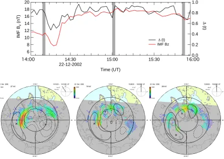
Fig. 2. Upper panel: IMFBz (red, axis on the left), as obtained by OMNI, and normalised disorder degree
Δ(t)(black, axis on the right) for the period 22/12/2002, 14:00 – 16:00 UT. Lower panel: three samples of
SuperDARN convection maps for the same period; the 2-minute scan intervals represented in the maps are shaded in the upper panel plot.
formation of single/multi scale spatial
fl
uctuations. If
Δ = 0
, we are in presence of a monocromatic
240
spectrum, so that the spatial
fl
uctuations are mainly characterised by a limited set of scales (in the
extreme case, by one scale only); conversely,
Δ = 1
corresponds to a
fl
at spectrum which is
associ-ated to multiscale
fl
uctuations. In this framework, complexity shows up in intermediate conditions,
i.e. when there is a certain number of
fl
uctuation scales interacting and evolving in time.
4 Results and Discussion
245We have applied the formalism described in the previous Sections to time series of PCP coef
fi
cients
as obtained from Eqs. 4 and 6 through the Ruohoniemi and Baker (1998) technique. The expansion
of the PCP has been limited to the fourth order, as we have checked that the results do not change
substantially if we use higher order expansions.
9
Fig. 2. Upper panel: IMFBz(red, axis on the left), as obtained by OMNI, and normalised disorder degree1(t )(black, axis on the right) for
the period 22/12/2002, 14:00–16:00 UT. Lower panel: three samples of SuperDARN convection maps for the same period; the 2-min scan intervals represented in the maps are shaded in the upper panel plot.
in this case, and are resampled in 60 2-min bins. The black curve displays the disorder degree1(t )calculated follow-ing the procedure described in the previous Section. The lower panel of Fig. 1 displays three 2-min snapshots of con-vection patterns as obtained from SuperDARN line-of-sight velocity data through the Ruohoniemi and Baker (1998) tech-nique; the scan intervals shown in the snapshots are evi-denced in the upper panel plot by gray-shaded areas. This first interval is characterised by a negative IMFBz: from the three patterns taken at the beginning of the period (19:30– 19:32 UT), at about a half of the period (20:30–20:32 UT) and at the end (21:28–21:30 UT), which are fully represen-tative of the whole event, a steady double cell configuration is evident, typical for such an IMF orientation (Ruohoniemi and Greenwald, 1996, 2005). The average value of1(t )is 0.35, evidencing that the ionospheric convection is charac-terised by a low disorder, where the information content con-tributing to1(t )is concentrated in a few spherical harmon-ics. After 21:05 UT1(t )starts to rise, reflecting changes in the convection patterns which lead the system towards more complex configurations; in fact, in the last snapshot on the right, in the lower panel of Fig. 1 (21:28–21:30 UT), we can see convection structures appearing around midnight MLT,
which perturb the quite regular two-cell symmetry that char-acterised the convection patterns before 21:00 UT.
Figure 2 shows data, in the same format as in Fig. 1, for the 22 December 2002, 14:00–16:00 UT interval, during which Bz was steadily positive. The upper panel displaysBz and 1(t ); the lower panel shows three snapshots of representa-tive convection patterns. Here the convection patterns show a double reverse cell configuration at high latitudes or, in gen-eral, strong fluxes of plasma directed sunward in the polar cap; at lower latitudes other convection cells show up, highly variable in size and dynamics. The main difference with re-spect to Fig. 1 is that1(t )is clearly higher, ranging between 0.6 and 0.9 and attaining the highest values after 14:40 UT, when the IMFBzexceeds 15 nT. It is natural to interpret this highly disordered configuration as an evidence of the contri-bution of a greater number of harmonics to the formation of the convection pattern. Moreover, we notice a qualitative cor-relation between1(t )andBz. Figure 3, upper panel, shows normalised histograms of1for all data points pertaining to Figs. 1 and 2, in red and blue for the scans of Figs. 1 and 2, respectively. The two1sets for negative and positiveBzare clearly separated, with only a small overlap around1=0.5. The negativeBz population peaks between 0.3 and 0.4 and
0.4
0.3
0.2
0.1
0.0
1.0 0.8
0.6 0.4
0.2 0.0
0.5
0.4
0.3
0.2
0.1
0.0
N/N
Tot
2003, 10, 01: Bz < 0 2002, 12, 22: Bz > 0
Fig. 3. Top panel: histograms of the normalised disorder degreeΔ, in 0.1 bins, for the October 1st, 2003,
19:30 – 21:30 UT (IMFBz<0, red cityscape) and December 22, 2002, 14:00 – 16:00 UT (IMFBz>0, blue
cityscape) intervals; the values of each histogram have been normalised to the total number of scans (which
is 60 for both). Bottom panel: second order complexity measureΓ11as a function of the normalised disorder
degreeΔfor the same time intervals (IMFBz<0: red dots; IMFBz>0: blue dots).
4.1 Case studies for different IMF orientations
250
Wefirst consider two two-hours intervals of SuperDARN data in the Northern Hemisphere,
charac-terised by almost steady conditions of the IMF and good overall coverage.
In Figure 1, upper panel, the IMFBz (red curve) is shown for the 19:30 – 21:30 UT period on
October 1st, 2003. IMF data come from the OMNI data base, in GSM coordinates in this case, and
are resampled in 60 2-minutes bins. The black curve displays the disorder degreeΔ(t)calculated
255
following the procedure described in the previous Section. The lower panel of Figure 1 displays three 2-minutes snapshots of convection patterns as obtained from SuperDARN line-of-sight velocity data through the Ruohoniemi and Baker (1998) technique; the scan intervals shown in the snapshots are
evidenced in the upper panel plot by gray–shaded areas. Thisfirst interval is characterised by a
negative IMFBz: from the three patterns taken at the beginning of the period (19:30 – 19:32 UT),
260
at about a half of the period (20:30 – 20:32 UT) and at the end (21:28 – 21:30 UT), which are
fully representative of the whole event, a steady double cell configuration is evident, typical for such
an IMF orientation (Ruohoniemi and Greenwald, 1996, 2005). The average value ofΔ(t)is 0.35,
evidencing that the ionospheric convection is characterised by a low disorder, where the information
10
Fig. 3. Top panel: histograms of the normalised disorder degree
1, in 0.1 bins, for the 1 October 2003, 19:30–21:30 UT (IMF
Bz<0, red cityscape) and 22 December 2002, 14:00–16:00 UT
(IMFBz>0, blue cityscape) intervals; the values of each histogram
have been normalised to the total number of scans (which is 60 for
both). Bottom panel: second order complexity measure011as a
function of the normalised disorder degree1for the same time
in-tervals (IMFBz<0: red dots; IMFBz>0: blue dots).
93% of its points fall below1=0.5, which means that in these cases the system tends to a more ordered configuration; on the other hand, the positiveBzpopulation peaks between 0.8 and 0.9 and 98 % of its points exceed 0.5, which corre-sponds to a high desorder degree. In the lower panel of Fig. 3 we show011plotted against1: red dots represent pairs of1 and011 values for theBz<0 interval, while blue dots re-fer to the scans of theBz>0 interval. As expected from its definition, the maximum complexity,011=0.25 is attained around1'0.5, i.e. corresponding to intermediate values of the normalised disorder parameter1. This presentation em-phasizes the fact that complexity is low both for high and for low values of1, which correspond to more disordered and more ordered convection configurations, respectively.
Around the complexity maximum, we find convection pat-terns which correspond to both positive and negative IMFBz. Figure 4 displays the time series of IMFBz(red curve) and the time series of1(black curve) for a period, 19 Decem-ber 2002, 06:00–10:00 UT, characterised by a variable IMF Bz. In fact,Bz was positive until about 07:32 UT, then be-came negative and switched again to positive values at about 08:52 UT. The values ofBz spanned from−15 up to 16 nT. Two vertical dashed lines mark the reversals of the sign ofBz in Fig. 4. One can see a correlation between the two curves:
-20 -10 0 10 20
IMF B
Z
[nT]
6:00 19-12-2002
7:00 8:00 9:00 10:00
Time (UT)
1.0
0.8
0.6
0.4
0.2
0.0
(t)
(t) IMF Bz
Fig. 4.Time series of IMFBz(red, axis on the left) in GSM coordinates, and normalised disorder degreeΔ(t)
(black, axis on the right) for the December 19th, 2002, 06:00 – 10:00 UT interval. The vertical black dashed
lines indicates the times whenBzchanges of sign, from positive to negative and vice versa.
rotations. By cross-correlating the two time series we have found that this time lag amounts to 10 min. Therefore, before building histograms as in the upper panel of Figure 3, we time–lagged the
Bzdata by 10 min (not shown).
Figure 5, upper panel, shows such histograms for the December 19, 2002, 06:00 – 10:00 UT event, 305
in the same format used for Figure 3, i.e. in red and blue for the positive and negativeBz scans,
respectively. In this case, the negativeBz population peaks between 0.4 and 0.5 and 70%of its
points fall belowΔ = 0.5, corresponding to the system collapsing towards order, while the positive
Bzpopulation peaks between 0.7 and 0.8 and 100%of its points exceed 0.5, which corresponds to
a high desorder degree. We can conclude that, in this case too, theΔhistograms for positive and
310
negativeBz are clearly separated, although the overlap of the two populations is somewhat greater
than in the case of Figure 3 and is slightly shifted towardΔ>0.5.
Figure 5, lower panel, showsΓ11 as a function ofΔfor the same interval above: again red dots
represent pairs of Δand Γ11 values for the scans characterised by negative IMFBz, while blue
dots are for pairs ofΔandΓ11 for positiveBz scans. Like for the two intervals shown in Fig. 3,
315
lower panel, also in this case we observe a mixing of ordered and disordered configurations across
the maximum of Γ11. Indeed, several points representing negativeBz configurations are rather
found on the right side of the curve, where the disorder degree is high. In this regard, we may add that, by careful visual inspection, we have found that such scans are mostly the ones closest
to the changes of sign of Bz and often correspond toBz values close to zero, both positive and
320
negative. Having said all that, we can consider the possibility that other parameters thanBzmay be
at play in determining the distribution of scan occurrence as a function ofΔ. In this regard, thefirst
possible candidate is obviously IMFBy, given its non-negligible role in the formation of ionospheric
convection cells. Actually,By does exhibit some variations in the time interval corresponding to
Figure 4. However, a 115 points statistics (about 4 hours of 2–minute radar scans) is too limited for 325
12
Fig. 4. Time series of IMFBz(red, axis on the left) in GSM
co-ordinates, and normalised disorder degree1(t )(black, axis on the
right) for the 19 December 2002, 06:00–10:00 UT interval. The
vertical black dashed lines indicates the times whenBzchanges of
sign, from positive to negative and vice versa.
1closely follows the IMFBzbehaviour, reaching high or in-termediate values whenBz is positive (maximum disorder), and taking lower values whenBz is negative (maximum or-der). We also notice that the1curve exhibits a lag relative to theBzcurve, which is particularly evident immediately after theBzrotations. By cross-correlating the two time series we have found that this time lag amounts to 10 min. Therefore, before building histograms as in the upper panel of Fig. 3, we time-lagged theBzdata by 10 min (not shown).
Figure 5, upper panel, shows such histograms for the 19 December 2002, 06:00–10:00 UT event, in the same for-mat used for Fig. 3, i.e. in red and blue for the positive and negativeBzscans, respectively. In this case, the negativeBz population peaks between 0.4 and 0.5 and 70 % of its points fall below1=0.5, corresponding to the system collapsing towards order, while the positive Bz population peaks be-tween 0.7 and 0.8 and 100 % of its points exceed 0.5, which corresponds to a high desorder degree. We can conclude that, in this case too, the1histograms for positive and negative Bzare clearly separated, although the overlap of the two pop-ulations is somewhat greater than in the case of Fig. 3 and is slightly shifted toward1 >0.5.
Figure 5, lower panel, shows011 as a function of1for the same interval: again red dots represent pairs of1 and 011values for the scans characterised by negative IMF Bz, while blue dots are for pairs of 1and011 for positiveBz scans. Like for the two intervals shown in Fig. 3, lower panel, also in this case we observe a mixing of ordered and disor-dered configurations across the maximum of011. Indeed, several points representing negative Bz configurations are rather found on the right side of the curve, where the disor-der degree is high. In this regard, we may add that, by careful visual inspection, we have found that such scans are mostly the ones closest to the changes of sign ofBzand often corre-spond toBzvalues close to zero, both positive and negative. Having said all that, we can consider the possibility that other
0.4
0.3
0.2
0.1
0.0
1.0 0.8
0.6 0.4
0.2 0.0
0.5
0.4
0.3
0.2
0.1
0.0
N/N
Tot
2002, 12, 19: Bz < 0 2002, 12, 19: Bz > 0
Fig. 5.Upper Panel: normalised histograms of the normalised disorder degreeΔ, in 0.1 bins, for the December
19th, 2002, 06:00 – 10:00 UT interval; red and blue cityscapes correspond to negative and positive IMFBz
scans, respectively. Values have been normalised to the total number of scans for eachBz polarity (69 and
46 for positive and negative values, respectively). Lower panel: second order complexity measureΓ11as a
function of the normalised disorder degreeΔfor same time interval.
a reliable characterisation of the relative roles of
B
zand
B
y. Hence, we perform such a study in the
next Section through the analysis of a much longer time period.
4.2 Study of an extended time interval
In this Section we will make use of a larger statistical sample of data in order to investigate the
combined in
fl
uence of IMF
B
zand
B
yon both complexity,
Γ
11, and disorder degree,
Δ
. For that
330
purpose, we selected a period of twenty days of SuperDARN data in the Northern Hemisphere,
during February 2002, on the grounds that this particular month is characterised by an abundant and
almost uniform data coverage and the IMF and the solar wind show a wide variety of conditions.
The time series of the three periods described in the previous Section have been added to the sample
as well.
335
For each of the 13604 SuperDARN 2–minute scans pertaining to the selected period, we
calcu-lated the 4th-order PCP coef
fi
cients and then calculated the
Δ
and
Γ
11parameters. As a second step
of the analysis, we calculated averages of
Δ
and
Γ
11(
Δ
,
Γ
11) in
[
B
z,B
y]
two dimensional bins
1
×
1
nT wide, from -15 up to 20 nT for both
B
zand
B
y. In order to avoid as much as possible
the effects of time lags like the one described in the case of Figure 4, the daily time series of the
340IMF
B
zhave been cross-correlated with the corresponding
Δ
time series and daily time lags have
13
Fig. 5. Upper Panel: normalised histograms of the normalised
dis-order degree 1, in 0.1 bins, for the 19 December 2002, 06:00–
10:00 UT interval; red and blue cityscapes correspond to negative
and positive IMFBz scans, respectively. Values have been
nor-malised to the total number of scans for eachBzpolarity (69 and 46
for positive and negative values, respectively). Lower panel:
sec-ond order complexity measure011as a function of the normalised
disorder degree1for same time interval.
parameters thanBzmay be at play in determining the distri-bution of scan occurrence as a function of1. In this regard, the first possible candidate is obviously IMF By, given its non-negligible role in the formation of ionospheric convec-tion cells. Actually,By does exhibit some variations in the time interval corresponding to Fig. 4. However, a 115 points statistics (about 4 h of 2-min radar scans) is too limited for a reliable characterisation of the relative roles ofBzandBy. Hence, we perform such a study in the next Section through the analysis of a much longer time period.
4.2 Study of an extended time interval
In this Section we will make use of a larger statistical sam-ple of data in order to investigate the combined influence of IMFBz andBy on both complexity, 011, and disorder de-gree, 1. For that purpose, we selected a period of twenty days of SuperDARN data in the Northern Hemisphere, dur-ing February 2002, on the grounds that this particular month is characterised by an abundant and almost uniform data cov-erage and the IMF and the solar wind show a wide variety of conditions. The time series of the three periods described in the previous Section have been added to the sample as well.
For each of the 13604 SuperDARN 2-min scans pertain-ing to the selected period, we calculated the 4th-order PCP
20
15
10
5
0
-5
-10
-15
IMF B
Z
GSM
[nT]
20 15 10 5 0 -5 -10 -15
IMF BY GSM
[nT]
0.8
0.7
0.6
0.5
0.4
0.3
0.2
20
15
10
5
0
-5
-10
-15
IMF B
Z
GSM
[nT]
20 15 10 5 0 -5 -10 -15
IMF BYGSM [nT]
0.24
0.22
0.20
0.18
0.16
Fig. 6.February 2002:Δ(upper panel) andΓ11(lower panel) as functions ofByandBz. The color scale
for each function is displayed on the right of each panel.
|By|/Bz1, a similar effect was found as a function of the IMFByintensity, so that bothBzand
Bymay be regarded as acting as control parameters.
The observed decrease of disorder for southward IMFBzhas to be related to the emergence of a
large scale coherence in the PCP structure manifesting in a more simple nearly two–cell structure. 380
Conversely, the higher degree of disorder for northward IMFBz conditions reflects the inherent
small scale multi–cell structure of ionospheric convection, which has to be associated with a reduced coherence in the large scale convection motions. It is in this framework that the transition from the small scale multi–cell structure of ionospheric convection for northward IMF condition to the nearly
two–cell structure observed for southward IMFBzis read as a dynamical order-disorder topological
385
phase transition, monitored by the changes inΔandΓ11.
In the recent literature (e.g. Sharma and Kaw, 2005; Consolini et al., 2008) it has been evi-denced how the overall magnetospheric dynamics is well in agreement with that of a system near a nonequilibrium stationary state displaying dynamical complexity. In such a scenario, the
topologi-15
Fig. 6. February 2002:h1i(upper panel) andh011i(lower panel)
as functions ofBy andBz. The colour scale for each function is
displayed on the right of each panel.
coefficients and then calculated the1and011 parameters. As a second step of the analysis, we calculated averages of 1 and 011 (h1i,h011i) in [Bz, By] two dimensional bins 1×1 nT wide, from−15 up to 20 nT for both Bz andBy. In order to avoid as much as possible the effects of time lags like the one described in the case of Fig. 4, the daily time series of the IMFBzhave been cross-correlated with the cor-responding1time series and daily time lags have been de-termined and applied to theBzdata. The average of such lag times is 16 min (±3 min). In order to exclude data with a too low statistical relevance, we dropped all averages pertaining to bins containing less than 10 scans. Figure 6 shows colour coded plots of such averages ofh1i(upper panel) andh011i (lower panel) as a function ofBzandBy. The results confirm and extend those for the case studies discussed above.
WhenBzis negative, the complexity measure is generally high (above 0.22 almost everywhere), assuming the high-est values whenByis dominant overBz. One could expect lower values ofh1iandh011iwhenBzis negative and dom-inant overBy, as we observed for example in the time period shown in Fig. 1; in this respect, we must say that the extended
time period we have chosen does not contain very long and steady intervals of strong negativeBz, so that we can specu-late that the system never really finds the favourable condi-tions for an “ideal” Dungey cycle activation. In such a case, a stable two-cell configuration should confine the informa-tion content in few harmonics, and the nearly maximum or-der for the system would be realised. In a more realistic pic-ture, frequentBzfluctuations continuously force the system in non-long standing stationary states, so increasing disorder and complexity.
The complexity decreases whenBz turns from negative to positive values: the ionospheric convection during posi-tiveBzperiods tends to configurations which show a strong topological disorder. Moreover, a broad region is evident for 0< Bz<10 nT and|By|/Bz<1, where 0.6<h1i<0.9 and complexity is low. We note also that in the same Bz do-main the increase of|By|tends to reduce the disorder and increase the complexity. Furthermore, a certain asymmetry in response to increasing IMFBy is observed: for positive IMFBz,h1iandh011iseem to increase more whenBy>0. One can conclude that, on a statistical basis, although the IMFBz<0 dominates the transition towards a more ordered (h1i<0.5) and complex configuration of the ionospheric convection, a similar effect is also due to IMF By when |By|/Bz1.
5 Conclusions
In this work we studied the reconfiguration of ionospheric convection from the point of view of information theory and complex system physics, so far not applied to such an is-sue. Starting from the Polar Cap Potential coefficients, as ob-tained from SuperDARN convection velocity data, we quan-titatively computed the pseudo Shannon entropy, the disor-der degree and the degree of complexity associated with the PCP structure on a global scale for three “paradigm” inter-vals first, and for an extended time period of about twenty days of data.
The obtained results clearly evidenced how the degree of complexity is a function of the IMF configuration. Indeed, a clear signature of a reduction of disorder and an increase of complexity is found when IMF turns from northward to southward. This behaviour can be interpreted in terms of a dynamical phase transition of the ionospheric convection pattern topology. Furthermore, when|By|/Bz1, a sim-ilar effect was found as a function of the IMFBy intensity, so that bothBzandBymay be regarded as acting as control parameters.
The observed decrease of disorder for southward IMFBz has to be related to the emergence of a large scale coher-ence in the PCP structure manifesting in a more simple nearly two-cell structure. Conversely, the higher degree of disorder for northward IMFBz conditions reflects the inherent small scale multi-cell structure of ionospheric convection, which
has to be associated with a reduced coherence in the large scale convection motions. It is in this framework that the transition from the small scale multi-cell structure of iono-spheric convection for northward IMF condition to the nearly two-cell structure observed for southward IMFBzis read as a dynamical order-disorder topological phase transition, mon-itored by the changes in1and011.
In the recent literature (e.g. Sharma and Kaw, 2005; Con-solini et al., 2008) it has been evidenced how the overall magnetospheric dynamics is well in agreement with that of a system near a nonequilibrium stationary state displaying dynamical complexity. In such a scenario, the topological phase transition, occurring during the increase of the global magnetospheric convection due to a southward turning of the IMF condition, is analogous to what occurs, for instance, in the case of Rayleigh-B´enard convection, when a long range coherence emerges out-of-equilibrium at high values of the overall temperature gradient and it is observed a reduction in the symmetry degree of the system. Paraphrasing the last concepts, we could say that the emergence of a long range coherence in the convection pattern during the southward turning of the IMF Bz component is a manifestation of a first-order like phase transition accompanied by a symmetry-breaking phenomenon.
The qualitative correlation between the1(t )and IMFBz time series, shown in Figs. 1, 2 and 4, and the apparent sys-tematic delay between the two curves deserve further inves-tigation in future studies, in order to explore the possibility of using1as a “quicklook” parameter of the overall iono-spheric convection.
Acknowledgements. This work is supported by the Italian Space
Agency (ASI) through the Exploration of Space System 2 program. The authors kindly aknowledge N. Papitashvili and J. King at the National Space Science Data Center of the Goddard Space Flight Center for the use permission of the 1-min IMF OMNI data and the NASA CDAWeb team for making these data available.
Edited by: P.-L. Sulem
Reviewed by: M. Leubner, Y. Elskens, and another anonymous referee
References
Abel, G. A., Freeman, M. P., and Chisham, G.: IMF clock an-gle control of multifractality in ionospheric velocity fluctuations, Geophys. Res. Lett., 36, L19102, doi:10.1029/2009GL040336, 2009.
Axford, W. I. and Hines, C. O.: A unifying theory of high-latitude geophysical phenomena and geomagnetic storms, Can. J. Phys., 39, 1433–1464, 1961.
Baker, K. B. and Wing, S.: A new magnetic coordinate system for conjugate studies at high latitudes, J. Geophys. Res., 94, 9139– 9143, 1989.
Burke, W. J., Kelley, M. C., Sagalyn, R. C., Smiddy, M., and Lai, S. T.: Polar cap electric field structures with a northward interplan-etary magnetic field, Geophys. Res. Lett., 6, 21–24, 1979.
Chang, T.: Low dimensional behaviour and symmetry breaking of stochastic systems near criticality – Can these effects be observed in space and in the laboratory?, IEEE T. Plasma Sci., 20, 691– 694, 1992.
Chang, T., Tam, S. W. Y., and Wu, C.–C.: Complexity in space plasmas – a brief review, Space Sci. Rev., 122, 281–291, 2006. Chen, J., Sharma, A. S., Edwards, J. W., Shao, X., and Kamide, Y:
Spatiotemporal dynamics of the magnetosphere during geospace storms: Mutual information analysis, J. Geophys. Res., 113, A05217, doi:10.1029/2007JA012310, 2008.
Chisham, G., Lester, M., Milan, S. E., Freeman, M. P., Bristow, W. A., Grocott, A., McWilliams, K. A., Ruohoniemi, J. M., Yeoman, T. K., Dyson, P. L., Greenwald, R. A., Kikuchi, T., Pinnock, M., Rash, J. P. S., Sato, N., Sofko, G. J., Villain, J.-P., and Walker, A. D. M.: A decade of the Super Dual Auroral Radar Network (Su-perDARN): scientific achievements, new techniques and future directions, Surv. Geophys., 28, 33–109, 2007.
Chisham, G., Freeman, M. P., Abel, G. A., Lam, M. M., Pinnock, M., Coleman, I. J., Milan, S. E., Lester, M., Bristow, W. A., Greenwald, R. A., Sofko, G. J., and Villain, J.-P.: Remote sens-ing of the spatial and temporal structure of magnetopause and magnetotail reconnection from the ionosphere, Rev. Geophys., 46, RG1004, doi:10.1029/2007RG000223, 2008.
Consolini, G., Marcucci, M. F., and Candidi, M.: Multifractal struc-ture of auroral electrojet index data, Phys. Rev. Lett., 76, 4082– 4085, 1996.
Consolini, G., De Michelis, P., and Tozzi, R.: On the
Earth’s magnetospheric dynamics: Nonequilibrium evolution and the fluctuation theorem, J. Geophys. Res., 113, A08222, doi:10.1029/2008JA013074, 2008.
Consolini, G., Tozzi, R., and De Michelis, P.: Complexity in the sunspot cycle, Astron. Astrophys., 506, 1381–1391, 2009. Cowley, S. W. H., and Lockwood, M.: Excitation and decay of
so-lar wind-driven flows in the magnetosphere-ionosphere system, Ann. Geophys., 10, 103–115, 1992,
http://www.ann-geophys.net/10/103/1992/.
De Michelis, P., Consolini, G., Materassi, M., and Tozzi, R.: An information theory approach to storm-substorm relationship, J. Geophys. Res., 116, A08225, doi:10.1029/2011JA016535, 2011. De Santis, A., Tozzi, R., and Gaya–Piqu´e, L. R.: Information content and K-entropy of the present geomagnetic field, Earth Planet. Sci. Lett., 218, 269–275, 2004.
Dungey, J. W.: Interplanetary magnetic field and the auroral zones, Phys. Rev. Lett., 6, 47–50, 1961.
Ebeling, W. and Klimontovich, Y. L. (Eds.): Self–organization and turbulence in liquids, Teubner-Verlag, Leipzig, Germany, 1984. Feller, W.: An introduction to probability theory and its
applica-tions, 3rd Edition, Vol. I, J. Wiley & Sons Inc., USA, 1970. Gosling, J. T., Thomsen, M. F., Bame, S. J., Elphic, R. C., and
Rus-sell, C. T.: Plasma flow reversals at the dayside magnetopause and the origin of asymmetric polar cap convection, J. Geophys. Res., 95, 8073–8084, 1990.
Greenwald, R. A., Baker, K. B., Dudeney, J. R., Pinnock, M., Jones, T. B., Thomas, E. C., Villain, J.-P., Cerisier, J.-C., Senior, C., Hanuise, C., Hunsucker, R. D., Sofko, G., Koelher, J., Nielsen, E., Pellinen, R., Walker, A. D. M., Sato, N., and Yamagishi, Y.: DARN/SUPERDARN: A Global View of the Dynamics of High-Latitude Convection, Space Sci. Rev., 71, 761–796, 1995.
Haken, H.: Synergetics, Introduction and Advanced Topics,
Springer-Verlag, Berlin, 2004.
Huang, C.-S., Andre, D. A., Sofko, G. J., and Koustov, A. V.: Super Dual Auroral Radar Network observations of ionospheric multi-cell convection during northward interplanetary magnetic field, J. Geophys. Res., 105, 7419–7428, 2000.
Klimas, A. J., Vassiliadis, D., Baker, D. N. and Roberts, D. A.: The organized nonlinear dynamics of the magnetosphere, J. Geophys. Res., 101(A6), 13089–13113, doi:10.1029/96JA00563, 1996. Klimontovich, Yu. L.: Turbulent Motion and the Structure of
Chaos, A new Approach to the Statistical Theory of Open Sys-tems, Kluwer Academic Publishers, Dordrecht, The Netherlands, 1991.
Klimontovich, Yu. L.: Criteria of Self-organization, Chaos Solut. Fractals, 5, 1985–2002, 1995.
Klimontovich, Yu. L.: Relative ordering criteria in open systems, Physics-Uspekhi, 39, 1169–1179, 1996.
Landsberg, P. T.: Thermodynamics and statistical mechanics, Ox-ford University Press, London, 1978.
Landsberg, P. T.: Can entropy and order increase togheter?, Phys. Lett. A, 102, 171–173, 1984.
Landsberg, P. T. and Shiner, J. S.: Disorder and complexity in an ideal non–equilibrium Fermi gas, Phys. Lett. A, 245, 228–232, 1998.
Lowes, F. J.: Mean-square values on sphere of spherical harmonic vector fields, J. Geophys. Res., 71, p. 2179, 1966.
Nicolis, G. and Nicolis, C: Foundations of Complex Systems, Non-linear Dynamics, Statistical Physics, Information and Prediction, World Scientific Publishing, Singapore, 2007.
Parkinson, M. L.: Dynamical critical scaling of electric field fluc-tuations in the greater cusp and magnetotail implied by HF radar observations of F-region Doppler velocity, Ann. Geophys., 24, 689–705, 2006,
http://www.ann-geophys.net/24/689/2006/.
Parkinson, M. L.: Complexity in the scaling of velocity fluctua-tions in the high-latitude F-region ionosphere, Ann. Geophys., 26, 2657–2672, doi:10.5194/angeo-26-2657-2008, 2008. Quian Quiroga, R., Arnhold, J., Lehnertz, K., and Grassberger,
P.: Kulback-Leinler and renormalized entropis: Applications to electroencephalograms of epilepsy patients, Phys. Rev. E, 62, 8380–8386, 2000.
Reiff, P. H. and Burch, J. L.: IMF By-dependent plasma flow and Birkeland currents in the dayside magnetosphere 2, A global model for northward and southward IMF, J. Geophys. Res., 90, 1595–1609, 1985.
Ruohoniemi, J. M. and Baker, K. B.: Large–scale imaging of high– latitude convection with Super Dual Auroral Radar Network HF radars observations, J. Geophys. Res., 103, 20797–20811, 1998. Ruohoniemi, J. M. and Greenwald, R. A.: Statistical patterns of high-latitude convection obtained from Goose Bay HF radar ob-servations, J. Geophys. Res., 101, 21743–21763, 1996.
Ruohoniemi, J. M. and Greenwald, R. A.: Dependencies
of high–latitude plasma convection: Consideration of inter-planetary magnetic field, seasonal, and universal time fac-tors in statistical patterns, J. Geophys. Res., 110, A09204, doi:10.1029/2004JA010815, 2005.
Sello, S.: Wavelet entropy as a measure of solar cycle complexity, Astron. Astrophys., 363, 311–315, 2000.
Sello, S.: Wavelet entropy and the multi–peaked structure of solar cycle maximum, New Astron., 8, 105–117, 2003.
Shannon, C. E.: A mathematical theory of communication, Bell Syst. Tech. J., 27, 379–423, 1948.
Sharma, A. S. and Kaw, P. K. (Eds.): Nonequilibrium phenomena in plasmas, Springer, Dordrecht, The Netherlands, 2005. Shepherd, S. G. and Ruohoniemi, J. M.: Electrostatic potential
pat-terns in the high latitude ionosphere constrained by SuperDARN measurements, J. Geophys. Res., 105, 23005–23014, 2000. Shiner, J. S., Davison, M., and Landsberg, P. T.: Simple measure of
complexity, Phys. Rev. E, 59, 1459–1464, 1999.
Sitnov, M. I., Sharma, A., Papadopoulos, K., Vassiliadis, D., Val-divia, J., Klimas, A., and Baker, D.: Phase transition-like behav-ior of the magnetosphere during substorms, J. Geophys. Res., 105, 12955–12974, 2000.
Sitnov, M. I., Sharma, A., Papadopoulos, K., and
Vassil-iadis, D.: Modeling substorm dynamics of the
magneto-sphere: From self–organization and self-organized criticality to nonequilibrium phase transitions, Phys. Rev. E, 65, 016116, doi:10.1103/PhysRevE.65.016116, 2001.
Wicks, R. T., Chapman, S. C., and Dendy, R. O.: Mutual infor-mation as a tool for identifying phase transition in dynamical complex systems with limited data, Phys. Rev. E, 75, 051125, doi:10.1103/PhysRevE.75.051125, 2007.