www.nonlin-processes-geophys.net/17/383/2010/ doi:10.5194/npg-17-383-2010
© Author(s) 2010. CC Attribution 3.0 License.
Nonlinear Processes
in Geophysics
Wave vector analysis methods using multi-point measurements
Y. Narita1, K.-H. Glassmeier1,2, and U. Motschmann3,4
1Institut f¨ur Geophysik und extraterrestrische Physik, Technische Universit¨at Braunschweig, Mendelssohnstr. 3, 38106 Braunschweig, Germany
2Max-Planck-Institut f¨ur Sonnensystemforschung, Max-Planck-Str. 2, 37191 Katlenburg-Lindau, Germany
3Institut f¨ur Theoretische Physik, Technische Universit¨at Braunschweig, Mendelssohnstr. 3, 38106 Braunschweig, Germany 4DLR-Institut f¨ur Planetenforschung, Rutherfordstr. 2, 12489 Berlin, Germany
Received: 24 June 2010 – Revised: 10 August 2010 – Accepted: 12 August 2010 – Published: 1 September 2010
Abstract. Recent developments of multi-point measure-ments in space provide a means to analyze spacecraft data directly in the wave vector domain. For turbulence study this means that we are able to estimate energy, helicity, and higher order moments in the wave vector domain without as-suming Taylor’s hypothesis or axisymmetry around the mean magnetic field. The methods of the wave vector analysis are presented and applied to four-point data of Cluster in the so-lar wind.
1 Introduction
Waves and turbulence observed in the interplanetary space and the Earth’s magnetosphere are one of the most interest-ing subjects in space physics, as plasmas allow various kinds of linear wave modes as excitation states to exist (that are well documented by, e.g., Stix, 1992 and Gary, 1993) and also various kinds of nonlinear waves and turbulent states (Biskamp, 2003). One of the complexities in plasma turbu-lence is that not only eddy splitting but also Alfv´en waves and other wave modes may be carriers of the energy cas-cade through wave-wave interactions. Earlier spacecraft ob-servations in 1960s revealed that magnetic field fluctuations in the solar wind are reminiscent of turbulence, as their fre-quency spectra often exhibited a power-law spectrum cha-racterized by the spectral index−5/3, the index known as Kolmogorov’s inertial-range spectrum for hydrodynamic tur-bulence. Regions upstream and downstream of Earth’s bow shock are also characterized by large-amplitude fluctuations, and they are thought to be in a turbulent state, too.
Correspondence to: Y. Narita
Earlier in-situ observations of space plasma turbulence were primarily limited to analyzing time series data based on single-spacecraft measurements, and the properties of the fluctuating magnetic field and flow velocity were deter-mined in the temporal or frequency domain. Investigation of spatial properties of the fluctuating fields relied on Tay-lor’s frozen-in flow hypothesis that neglects wave frequen-cies in the flow-rest frame when a fluctuating field is sampled in a fast-streaming medium (Taylor, 1938). This hypothe-sis relates the observed frequency with the wave number in the flow direction using the Doppler shift,ω'k·V, where ω is the spacecraft-frame frequency, and k and V are the wave vector and the flow velocity vector, respectively. The solar wind is a fast-streaming plasma with the Mach num-ber being 8 to 10 with respect to the sound speed and also the Alfv´en speed. Therefore, Taylor’s hypothesis is believed to be valid and has been widely applied in studying solar wind turbulence (Coleman, 1968; Matthaeus and Goldstein, 1982; Marsch and Tu, 1990; Podesta et al., 2007). Other physical quantities relevant to plasma turbulence such as the magnetic helicity density, the cross helicity, and the Els¨asser variable spectra were also determined by adapting and reduc-ing these quantities to the context of sreduc-ingle-spacecraft mea-surements (Matthaeus and Goldstein, 1982; Matthaeus et al., 1982; Glassmeier et al., 1989; Marsch, 1991; Tu and Marsch, 1995).
achieved in early single-point measurements because the Doppler shift was not corrected. Spatial properties of the fluctuating fields can be determined only by multi-point mea-surements: They allow us to determine the wave vectors, the wave propagation speeds and directions, the rest-frame fre-quencies by correcting the Doppler shift, and the fluctuation amplitudes associated with the wave vectors and the rest-frame frequencies. Furthermore, multi-point measurements also provide the opportunity to verify Taylor’s hypothesis.
This paper reviews the wave vector analysis methods de-veloped particularly for the Cluster mission (Escoubet et al., 2001; Balogh et al., 2001) to make use of full potential of the four-point measurements in space. Examples include (1) the wave telescope technique, (2) the extended wave telescope technique, and (3) the eigenvector analysis methods. The mathematical foundation of these methods are explained as well as application to the Cluster data. The wave telescope technique performs a parametric projection of the measured fluctuations into the wave vector domain and does not re-quire any knowledge on dispersion relations nor Taylor’s hy-pothesis. Using this technique and its extended methods, the distributions of energy and helicity can be determined in the frequency-wave vector domain. From the 3-D energy distribution, Taylor’s hypothesis is verified for the first time for solar wind turbulence. Also, the analysis of bispectrum can be performed in the wave vector domain using the wave telescope technique. The concept of bispectrum represents a triple correlation that measures occurrence or strength of wave resonance processes among three different wave com-ponents, and therefore it serves as a useful analysis tool to in-vestigate energy cascade process in turbulence. Details about the bispectrum analysis are explained in Sect. 3.3. The eigen-vector analysis is another approach in wave analysis and pro-vides methods to determine dispersion relations and high-resolution wave number spectra.
2 Projection methods
It is of course ideal to have as many properly positioned spacecraft available as possible to Fourier transform ob-served fluctuations from the spatial coordinates into the wave numbers. The four measurement points of Cluster, from this point of view, are too few for performing a Fourier transform into the wave number domain, but it was proposed to esti-mate the energy distribution in the 4-D frequency-wave vec-tor domain using four point measurements only. The idea to use multiple spacecraft as a plasma wave array experiment was originally raised by Musmann et al. (1974) before the concept of the Cluster mission was developed. The idea of the array experiment using multi-spacecraft was further de-veloped for the Cluster mission (Neubauer and Glassmeier, 1990; Pinc¸on and Lefeuvre, 1991; Motschmann et al., 1996; Glassmeier et al., 2001), applying the projection methods
earlier used in seismic wave studies (Capon, 1969; Harjes and Henger, 1973).
We define the state vector for anL-point measurements as
S(ω)=
S(ω,r1) S(ω,r2)
.. . S(ω,rL)
. (1)
Here each sensor measures a scalar quantitySat thei-th po-sition of the sensorsri. The fieldSis already transformed from the time into the frequency domain, and is a function of the frequencyωand the positionri. Consider a projection of the state vector, which provides the amplitude as a func-tion of the frequency and the wave vector. In other words, the state vector is reduced to a scalar by taking a dot product with a suitable weight or projection vector. We measure a scalar field using a sensor-array and determine the state vector in the frequency domain; and then the state vector is reduced to a scalar. The projected quantity is the wave amplitude given as a complex number, retaining the phase information in the frequency-wave vector domain:
S (ω,k)=w†(ω,k)·S(ω), (2) wherew†(ω,k)denotes the weight vector or the projection vector (the dagger means Hermitian conjugate). One may also estimate the wave power in the frequency-wave vector domain as:
P (ω,k)= h|S (ω,k)|2i =w†(ω,k)R(ω)w(ω,k), (3) where R(ω)denotes theL-by-Lcross spectral density (CSD) matrix determined by the state vector:
R(ω)= 1 T D
S(ω)S†(ω)E. (4)
The factor 1/T represents a division by the measured time lengthT, so that the elements of the CSD matrix are given as energy density in the frequency domain, in units of squared amplitude per frequency. The angular bracket h···i repre-sents the operation of averaging. We use in our data analysis the time averaging, assuming that fluctuations are stationary. The task is now to find the weight vector in a suitable form describing the amplitude or the power associated with the pa-rameterk, the wave vector. We introduce two different pro-jection methods: beam-former propro-jection and Capon’s mini-mum variance projection.
2.1 Beam-former projection
Let us define the steering vector that describes a plane wave approximation characterized by the wave vectork:
h(k)=
eik·r1
eik·r2
.. . eik·rL
The beam-former projection uses the steering vector as the weight vector,
w=h, (6)
and the wave power is estimated as
PBF=h†Rh. (7)
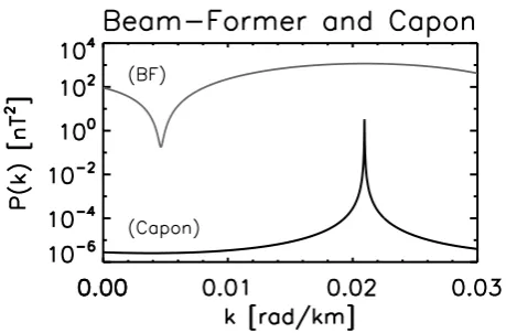
An example of the wave number spectrum evaluated with the beam-former projection technique is displayed in Fig. 1 for synthetic data. In this example, a single plane wave is gen-erated with the wave numberk=0.021 rad/km and the fluctu-ating field is sampled at four distinct points in a 1-D array as time series data. The evaluated spectrum shows a max-imum at the signal wave number, but the spectrum is very broad and flat and identification of the signal wave number under the high background level in the spectrum is difficult. Furthermore, the spectrum exhibits a drop at relatively small wave numbers. The result is therefore much different from the spectrum of the synthetic data.
2.2 Capon’s minimum variance projection
To reduce the high background level of the beam-former spectrum and to make the spectrum have a sharp peak at the signal wave vector, Capon (1969) proposed the method of minimum variance projection. Consider minimizing the power while keeping the fluctuation amplitude at the look-ing wave vectork unchanged (referred to as the unit gain constraint). The task is to minimize the interference in the spectrum that come from wave vectors other than the looking wave vector. This problem can be formulated as an optimiza-tion problem under a constraint as follows:
minimize w†Rw subject to w†·h=1 or
δ h
w†Rw−λ
w†·h−1i=0, (8)
with the Lagrangian multiplierλ. Capon (1969) obtained the analytical solution for this problem as follows:
w= R
−1h
h†R−1h. (9)
The projected power is therefore PC= 1
h†R−1h. (10)
See, for example, Haykin (1991) for the derivation. It is worthwhile to note that Capon’s projection vector is deter-mined not only by the steering vector but also by the mea-surement itself through the state vector. An example of the spectrum evaluated by Capon’s method is presented in Fig. 1 for the same data as that used for the beam-former spectrum. The Capon spectrum shows a much clearer peak at the sig-nal wave number and the background level is significantly reduced.
Fig. 1. Wave number spectra evaluated by the beam-former (BF)
and Capon’s projection methods.
2.3 Wave Telescope Technique
The projection method can be generalized to measurements of vectors such as the magnetic field, and the state vector has 3L elements (3 components of the vector measured by Lsensors). In the case of the Cluster magnetometer data the number of sensor isL=4, and the state vector is established as:
S(ω)=
B1(ω)
B2(ω) .. .
B4(ω)
, (11)
and the generalized CSD matrix is R(ω)= 1
ThS(ω)S
†(ω)i. (12)
The CSD matrix is a 3L×3Lmatrix and depends on the fre-quency. After the projection, the CSD matrix is reduced to a 3×3 matrix, and each element of the matrix represent the correlation among thex,y, andzcomponent of the fluctu-ating magnetic field as a function of the frequency and the wave vector. The steering vector is a 3L×3 matrix:
H(k)=
Ieik·r1
Ieik·r2
Ieik·r3
Ieik·r4
, (13)
where I denotes the 3×3 unit matrix. The formula of Capon’s projection can be generalized to matrix operations, and we obtain the projection matrix as (Pinc¸on and Lefeuvre, 1991; Motschmann et al., 1996)
W=R−1HhH†R−1Hi
−1
(14) under the unit gain constraint:
The projected matrix is expressed as: P=
h
H†R−1Hi
−1
. (16)
This is a 3×3 correlation matrix in the frequency-wave vec-tor domain. The diagonal and off-diagonal elements repre-sent the fluctuation power and wave helicity, respectively. The trace of the matrix gives the total fluctuation power.
In addition, one may impose an additional constraint that the field satisfies the divergence-free condition (Pinc¸on and Lefeuvre, 1991; Motschmann et al., 1996). This can be ex-pressed as
k·W†S=0. (17)
This condition may be reflected to the state vector S such thatS is replaced by VS, where the matrix V represents a projection of the state vector onto the plane perpendicular to the wave vector:
V=I+kk
k2. (18)
The matrix V can be directly incorporated in Capon’s spec-trum and we obtain the projection matrix as
W=R−1HVhV†H†R−1HVi
−1
(19) and the projected matrix:
PWT=hV†H†R−1HVi
−1
. (20)
The trace of the projected matrix gives the total fluctuation power at frequencyωand the wave vector k:
PWT=tr
h
V†H†R−1HVi
−1
. (21)
Estimating the power in the wave vector domain using the three matrices R, H, and V is called the wave tele-scope technique or k-filtering (Pinc¸on and Lefeuvre, 1991; Motschmann et al., 1996; Glassmeier et al., 2001; Pinc¸on and Motschmann, 1998; Pinc¸on and Glassmeier, 2008), and it provides the means to determine the energy distribution in the 4-D frequency-wave vector domain using Cluster data. Note that the projection vectorwand the projection matrix W are the dimensionless operators and they do not change the units of the spectrum after the projection, i.e., the same dimension as the CSD matrix (squared amplitude per fre-quency). A suitable procedure is needed to properly evalu-ate Capon’s spectra as energy distributions or energy density spectra. After integration of Capon’s spectra over frequen-cies the spectra are given in units of power (squared ampli-tude), and the division by the wave number interval after the integration the spectra are adapted to the energy density spec-tra in units of squared amplitude per wave number.
An example of the 3-D energy distribution in the wave vector domain evaluated by the wave telescope technique is displayed in Fig. 2. In this example, synthetic time series data are generated from the model energy distribution (which is an isotropic distribution in the wave vector domain) with random phases. The fluctuations are sampled at four dis-crete points forming a tetrahedron. The energy distribution is then reconstructed from four-point time series data using the wave telescope technique. Although the reconstructed distri-bution is not exactly the same as the model distridistri-bution, the overall structure can be reasonably well reconstructed (Narita et al., 2010a). The wave telescope technique has the advan-tage that it does not require any knowledge on the number of signals. In the MUSIC algorithm (presented later), one has to know the number of signals. It is worthwhile to note that Capon’s projection method is valid not only for plane waves but also for other spatial structures. Constantinescu et al. (2006, 2007) generalized the wave telescope technique for spherical wave patterns. Plaschke et al. (2008) generalized it to field-line-resonant phase patterns of ULF pulsations of the geomagnetic field using phase-shifted waves. The associated spatial patterns are displayed in Fig. 3.
Fig. 2. Comparison of energy distribution in the 3-D wave vector domain. Left panel displays the model distribution from which synthetic
data are generated and sampled at four different positions in the spatial coordinate. Right panels displays the energy distribution reconstructed using the wave telescope technique. Adapted from the numerical test of the wave telescope technique in Narita et al. (2010a).
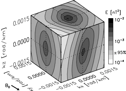
As an application to the Cluster data, Fig. 4 displays the 3-D energy distribution in the wave vector domain for mag-netic field fluctuations in the solar wind. The energy distri-bution is determined in the 4-D frequency-wave vector do-main in the spacecraft frame, and then the Doppler shift is corrected and the distribution is transformed into the flow rest frame. Finally, the 4-D distribution is reduced to the 3-D distribution by integrating over the rest-frame frequen-cies. The distribution is anisotropic and exhibits an extended structure perpendicular to the mean magnetic field direction, suggesting that the observed solar wind fluctuations repre-sent the geometry of quasi-2-D turbulence. While earlier measurements based on single-point measurements already revealed the anisotropy in solar wind turbulence, Taylor’s hy-pothesis and axisymmetry around the mean field had to be assumed to infer the energy distribution in three-dimension (Matthaeus et al., 1990; Carbone et al., 1995; Dasso et al., 2005). The wave telescope technique does not require such assumptions and determines the 3-D energy distribution di-rectly in the wave vector domain. One of the most important conclusions of the 3-D energy distribution is that the turbu-lence in solar wind is not axisymmetric about the background magnetic field (Narita et al., 2010c). This was not seen be-fore the Cluster mission. Various interpretations are possible to explain the non-axisymmetric structure: it may originate in the coronal magnetic field structure, or perhaps it is caused by the radial expansion of solar wind. Statistical study of the 3-D energy distributions on various spatial scales would be a suitable task for this problem, which is being carried out currently.
It is furthermore possible to verify Taylor’s hypothesis us-ing the 3-D energy distribution. The 1-D energy spectrum is estimated by reducing the 3-D distribution into 1-D wave number domain in the flow direction and transforming it into the energy density in the wave number domain (in units of
Phase-shifted plane wave
Plane wave Spherical wave
Fig. 3. Spatial patterns that can be used for the Capon’s projection
technique, after Constantinescu (2007).
Fig. 4. Cubic representation of magnetic energy distribution in the
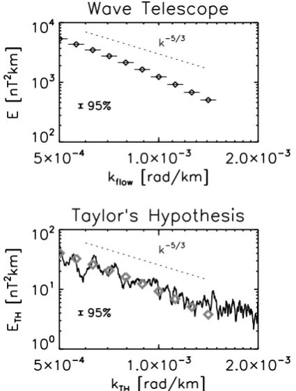
squared amplitude per wave number interval). The energy spectrum in the flow direction is then compared with that evaluated using Taylor’s hypothesis in Fig. 5. The spectrum estimated from the wave telescope technique (upper panel) shows deviation from the power-law spectrum with the index −5/3 at larger wave numbers. The spectrum estimated from Taylor’s hypothesis (lower panel) can be fitted on the whole by a power-law with the index−5/3, but the spectrum shows deviations (or fluctuations) from the power-law curve at var-ious wave numbers. The direct comparison between the two spectra suggests that Taylor’s hypothesis appears to be valid, but one should keep in mind that the resolution of the wave numbers is not very satisfactory in the reduced spectrum (up-per panel), and further investigations would be needed to ver-ify on what scales Taylor’s hypothesis clearly breaks down. Taylor’s hypothesis neglects wave frequencies in the flow-rest frame compared to the Doppler term, the breakdown of Taylor’s hypothesis is expected when the rest-frame frequen-cies cannot be neglected. Another possibility of the break-down of Taylor’s hypothesis is that there is no dispersion re-lation in the fluctuations and the energy distribution spreads both in the frequency and wave vector domain, such that higher frequencies in the flow-rest frame contribute signifi-cantly as well as lower frequencies. Therefore, whether or not a dispersion relation exists and how the energy spectrum in the rest-frame frequency domain looks like are very impor-tant questions in turbulence. The energy spectra in the wave vector domain are evaluated for magnetic field fluctuation in various regions: in the solar wind (Narita et al., 2010a,b,c), foreshock (Narita et al., 2006; Narita and Glassmeier, 2010d) and magnetosheath (Sahraoui et al., 2003, 2006; Narita and Glassmeier, 2010d).
3 Extended wave telescope technique 3.1 Magnetic helicity density
The wave telescope technique provides a 3×3 matrix with each element representing a correlation amongBx,By, and Bzcomponents of fluctuations in the frequency-wave vector domain. While the diagonal elements of the CSD matrix rep-resent the wave power, the off-diagonal elements reprep-resent cross-correlations and contain information about the mag-netic helicity density. To relate the projected CSD matrix with the magnetic helicity density, we use the expression of the vector potentialafor the fluctuating magnetic fieldb:
a= −i
k2k×b. (22)
The magnetic helicity density can be determined by build-ing a scalar product between the vector potentialaand the magnetic fieldb:
hM= ha†·bi, (23)
where the angular bracketh···irepresents the averaging over different ensembles, e.g., averaging over different time
se-Fig. 5. Comparison of the wave number spectra. The upper panel
is the energy spectrum for the wave number in the flow direction, reduced from the 3-D energy distribution using Cluster data and the wave telescope technique. The lower panel displays the energy spectrum transformed from the frequency into the wave number do-main using Taylor’s hypothesis (solid line) and the reduced spec-trum shown in the upper panel (squares) with adjustment for com-parison of the spectral slope.
ries data. The magnetic helicity density is related to the off-diagonal elements of the projected CSD matrix as (Narita et al., 2009b):
hM=− i k2
kx(Pyz−Pzy)+ky(Pzx−Pxz)+kz(Pxy−Pyx)
.
(24) It is worthwhile to note that the estimate of the helicity den-sity Eq. (24) is constructed as gauge-independent, and it is evaluated in the frequency-wave vector domain.
Fig. 6. Energy and helicity density in the frequency-wavenumber
domain for a synthetic data set of four-point measurements of mag-netic field (Narita et al., 2009b).
kind of polarization or helicity (i.e., linear, circular, and el-liptical polarization), the helicity distribution shows the ac-tivities for the circular or elliptical sense of field rotation. The peaks are located on the positive wave number side, pa-rallel to the mean magnetic field and it is also in the direc-tion away from the shock to the interplanetary space. From the rest-frame frequencies and the wave numbers one may estimate the phase speeds, and they are aboutvph=40 km/s andvph=88 km/s atk=0.0010 rad/km and k=0.0017 rad/km, respectively. The latter peak is close to the Alfv´en speed of the background plasma, about 77 km/s, while the first one is about half of the Alfv´en speed. Figure 6 suggests that the foreshock waves represent the growth of ion instabilities driven by ion beams moving sunward from the shock. The energy and magnetic helicity distributions in the frequency-wave number domain essentially agree with the predictions based on the wave kinetic theory (Gary, 1993).
3.2 Wave telescope for flow velocity data
Although the wave telescope technique was developed par-ticularly for analyzing multi-point magnetic field data, it can be applied to to the multi-point flow velocity data. For exam-ple, Cluster electron data are available at four spacecraft and the data is suitable for the wave telescope analysis. However, the divergence-free condition is not always valid for flow
ve-locity fields and the wave telescope technique for the flow velocity should use the form of Eq. (16). In a similar fashion to the approach used in the magnetic helicity density, various quantities relevant to fluid turbulence may be evaluated using the flow velocity data. The kinetic energy is the trace of the projected CSD matrix, and the off-diagonal elements of the matrix provide the kinetic helicity densityhK= hu·i. The symboldenotes the vorticity, the curl of the flow velocity. The kinetic helicity density is related to the projected CSD matrix as:
hK=Du†·E (25)
=ikx(Pu,yz−Pu,zy)+ky(Pu,zx−Pu,xz)
+kz(Pu,xy−Pu,yx). (26) In this expression we used the vorticity in the Fourier do-main:
=ik× ˜u, (27)
where the tilde-hat represents the Capon projection into the frequency-wave vector domain, and Pu,ij denotes the the (i,j )-component of the projected CSD matrix for the flow velocity. It is also possible to evaluate the enstrophy (the squared vorticity) and the dilatation (the divergence of the ve-locity, which is a measure of the fluid compressibility). The former is given as
2= |k× ˜u|2, (28)
and the latter is
d2= |k· ˜u|2, (29)
Finally, the correlation between the flow velocity and the magnetic field gives the cross helicity density,hC= h ˜u†· ˜bi. This can be evaluated in the frequency-wave vector domain, too.
3.3 Higher order moments
Using the wave telescope technique it is possible to esti-mate higher order moments which are useful quantities to study wave-wave interactions. For example, third order mo-ments (also named bispectra or three-point correlations) are the measure of three-wave couplings and can be determined in the frequency-wave vector domain. Three-wave processes are characterized by the resonance condition of frequencies and wave vectors, described asω00=ω±ω0andk00=k±k0. One of the third order moments relevant in plasma physics the triple correlation of two fluctuation components of the magnetic field and a density fluctuation component under the conditionsω00=ω+ω0andk00=k+k0:
F ω,ω0,k,k0
=b(ω,k)n ω0,k0
projected into the frequency-wave number domain using Capon’s method:
b(ω,k)=w†b(ω,k)·Sb(ω) (31) n(ω,k)=w†n(ω,k)·Sn(ω). (32) HereSb(ω)andSn(ω)are the state vectors of the magnetic field and the number density, and wb and wn are the re-spective projection vectors. The asterisk denotes the oper-ation of complex conjugate. The meaning of the bispectrum is as follows. If three waves are in resonance in the mea-sured data, the bispectrum returns a non-zero quantity, other-wise the bispectrum for the other non-resonant waves returns a small value close to zero due to the averaging operation. The bispectrum can be investigated for the plus-sign coupling (ω+ω0andk+k0) and for the minus-sign coupling (ω−ω0 andk−k0).
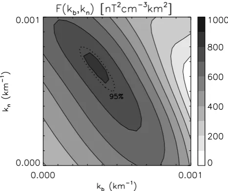
The bispectrum was evaluated using Cluster data in the wave vector domain for the couplingkb+kn=k0b (Fig. 7), wherekb andkn denote the wave numbers of the fluctuat-ing magnetic field and the electron density, respectively. The primed wave vector k0b is another wave vector of the fluc-tuating magnetic field. The data are taken from the Cluster observation in the foreshock region. The bispectrum is eval-uated at various combinations ofkb andkn using the reso-nance condition, and its distribution exhibits a peak at one particular combination of these two wave vectors.
The magnetic field and the electron data were used for the bispectral analysis for the following reason. There are various types of wave-wave interactions proposed in plasma physics, and one of them describes the interaction of an Alfv´en wave (that is a fluctuation in the magnetic field) with a sound wave (that is a density fluctuation), generating another Alfv´en wave at the resonant frequency and wave vector. The decay and the modulational instabilities belong to this fam-ily of interaction (Derby, 1978; Goldstein, 1978; Longtin and Sonnerup, 1986; Mjølhus, 1976; Spangler, 1999; Terasawa et al., 1986; Wong and Goldstein, 1986). The displayed ex-ample does not immediately imply an evidence of these in-stabilities in space plasma observation, but suggests that such an analysis can be performed both in the frequency and in the wave vector domain, which provides a means to study, either to prove or to disprove, these instabilities using spacecraft data. It is worth noting that Fig. 7 not only provides the direct evidence of wave-wave resonance in the spatial domain but also suggests that the parametric instability of Alfv´en wave may be occurring in the foreshock region, in which an Alfv´en wave collapses into another Alfv´en wave and a density fluc-tuation (e.g., sound wave). However, more careful studies are needed to confirm the existence of parametric instability, for example, by investigating the bispectrum in the both fre-quency and wave vector domain; comparing the background condition such as the plasma beta with the theoretical predic-tions.
Fig. 7. Bispectrum using magnetic field and electron density data
of Cluster in the foreshock under the resonancekb+kn, wherekb
andknrepresent the wave number of the fluctuating magnetic field
and electron density parallel to the mean magnetic field. The dotted line denotes the level of 95 % confidence (Narita et al., 2008).
4 Eigenvector analysis
The CSD matrices of the state vectors are Hermitian-symmetric and they may be decomposed into a set of eigen-values and eigenvectors, which have information about spa-tial structure of waves. Investigation of the eigenvectors of the CSD matrix represents provides another useful wave vec-tor analysis tools. We present in this section two applica-tions: the wave surveyor technique (Vogt et al., 2008) and the multi-point signal resonator (MSR) technique (Narita et al., 2010b). The former provides a wave vector identification method for the dominant wave components and the latter pro-vides a high-resolution wave number spectrum.
4.1 Wave surveyor technique
observer’s frame. We therefore minimize the deviation or difference between the ideal phases and the measured phases, i.e., minimize the following function
Q(k,φ)= L X
i=1
[θi−k·ri−φ]2, (33)
with respect to the wave vectorkand the initial phaseφ. It can be shown that the wave vector can be directly obtained from the eigenvector phases as (Vogt et al., 2008):
k= X
i
rirti !−1
X
i
θiri. (34)
Herert is the transposed vector of the sensor positions mea-sured from the center of the sensor array. The position vec-tors satisfy the conditionP
iri=0. In the case of four sen-sors (L=4) like the Cluster mission, the solution can be given as a linear combination of the reciprocal vectors of the spacecraft positionsκi (Neubauer and Glassmeier, 1990; Chanteur, 1998),
k(ω)= 4 X
i=1
θi(ω)κi. (35)
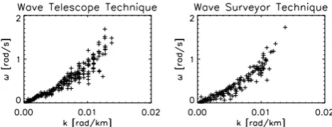
This method directly determines the wave vector associated with the frequencyωis called the wave surveyor technique (Vogt et al., 2008). The wave surveyor technique gives a very similar result in the dispersion relation analysis to that of the wave telescope technique. Figure 8 displays the comparison of the dispersion relation for foreshock waves measured by Cluster. The dispersion relations in Fig. 8 agree with the theoretical prediction of ion beam instability (Gary, 1993), and therefore comfirm that the foreshock waves are driven by the backstreaming ion beams from the shock.
4.2 MUSIC algorithm and MSR technique
The eigenvectors of the CSD matrix are strictly orthogo-nal to one another, and this fact can be used for establish-ing another estimator of the wave number spectrum. The MUSIC algorithm (Multiple SIgnal Classification) was pro-posed by Schmidt (1986) on the assumption that the mea-sured data contains signal and noise such that the CSD matrix can be decomposed into two parts. The state vec-tor is therefore interpreted as a combination of the signal term and the noise term. Under this concept the CSD ma-trix is decomposed into the signal term and the noise term, too. The eigenvalues and eigenvectors of R are denoted byλ1≥λ2≥ ··· ≥λL ande1,e2,···,eL, respectively. For the noise part the eigenvalues are given as the “noise floor” (Haykin, 1991) such thatλM+1=λM+2= ··· =λL=σ2. We split the eigenvectors of the CSD matrix R into two parts: the signal subspace Es= [e1,e2,···,eM]and the noise subspace En= [eM+1,eM+2,···,eL].
Fig. 8. Dispersion relation of foreshock waves measured by Cluster.
Left panel displays the dispersion relation determined by the wave telescope technique (Narita et al., 2007), and right panel displays that determined by the wave surveyor technique (Vogt et al., 2008). Wave numbers are in the direction to the mean magnetic field and frequencies are given in the flow rest frame after the Dopper correc-tion.
The power estimation in the MUSIC method is given as PMUSIC=
1 |h†En|2
(36)
= 1
h†EnE†nh
, (37)
which makes use of the orthogonality between the steering vectorh(ki)(i=1,···,M) and the eigenvector for the noise partej (j=M+1,···,L):
h†(ki)·ej=0. (38)
The MUSIC spectrum is also expressed using all eigenvec-tors as
PMUSIC= 1
h†FLF†h, (39)
where F is the eigenvector matrix of R sorted in descending order of the eigenvalues
F= [EsEn] =e1···eM eM+1···eL. (40) The matrix F is an arrangement of the eigenvectors of the CSD matrix, placing the signal-associated eigenvectors on the left side in the matrix and the noise-associated eigenvec-tors on the right side. The matrix L is a diagonal matrix and is defined as
L=diag
0,···,0 | {z }
M
,1,···,1 | {z } L−M
. (41)
be noted that the MUSIC algorithm requires that the number of signals must be known in the analysis to extract the set of the eigenvectors associated with noise. One method to deter-mine the number of signals is to investigate the noise floor of the eigenvalues, for example, in a plot of eigenvalues in descending order (Haykin, 1991).
The problem that the number of signal sources must be known in the MUSIC algorithm was solved by Choi et al. (1993) by replacing the diagonal matrix L by3−nwith
3−n=diag λ
1 λL
−n ,
λ 2 λL
−n ,···,
λ L λL
−n!
. (42)
Here the power−nis an adjustable parameter (n=1,2,···) in the analysis that controls the asymptotic behavior of the estimator such that the matrix3−n becomes L in the limit n→ ∞. In other words, replacing the matrix L by3−n au-tomatically selects the noise subspace of the CSD matrix R. It should be noted that the procedure of the matrix replace-ment by3−n does not stem from any mathematical theory guaranteeing better functionality of the technique, but it rep-resents an intuitive picture of generalization of the matrix L to soften its sharp transition of the diagonal elements from zero to one. Therefore, other extensions or generalizations are possible for the MUSIC algorithm. Choi et al. (1993) found that even a small number ofnsuch asn=2 can suc-cessfully reproduce the MUSIC spectrum without knowing the number of signal sources. The spectrum using the ex-tended MUSIC algorithm is given as
PEM= 1
h†F3−nF†h. (43)
The spectrumPEMis given in the dimensionless unit, but it may be used as a filter to Capon’s spectrum. The MSR technique (Multi-point Signal Resonator) makes use of this notion to establish an estimator of high-resolution wave num-ber spectra: We use Capon’s estimator and obtain the power spectrum that exhibits the right value of the spectrum at the signal wave number; and we use additionally the extended MUSIC spectrum with a proper normalization as a dimen-sionless filter to enhance the signal-to-noise contrast of the Capon spectrum. The power spectrum in the MSR technique is therefore given as
PMSR= 1
PEM0PEMPC. (44)
Here the factor 1/PEM0 denotes normalization of the ex-tended MUSIC spectrum, and is a sum of the exex-tended- extended-MUSIC spectrum over the frequency-wave vector domain:
PEM0= X
ω,k
PEM(ω,k). (45)
The normalized, extended MUSIC spectrum PEM(ω,k)/PEM0 serves as a filter that returns the value
Fig. 9. Capon and MSR spectra for the synthetic data with two wave
components that have similar or very close wavelengths (Narita et al., 2010b).
of almost one at the signal wave numbers and almost zero values otherwise, which enhances the quality of Capon’s spectrum. Another merit of the MSR technique is that it can resolve waves with slightly different wavelengths or wave numbers. Figure 9 displays the spectral curves determined by the Capon and the MSR technique for a synthetic data set in which two wave components have close wave numbers to each other. The MSR spectrum can resolve two peaks at the signal wave numbers, whereas Capon’s spectrum exhibits a peak with broadening. The peak at the smaller wave number in the MSR spectrum appears as a hump in the Capon spectrum, and identification of this peak is difficult. This example shows the ability of the MSR technique: much reduced background level; and high-resolution in the wave vector domain. The MSR technique can also be used for a measurement of a vector quantity such as the magnetic field. It is also possible to set the divergence-free condition as an additional constraint. Details of the MSR technique are discussed in Narita et al. (2010b).
5 Conclusions
separation and configuration phases in its operation, rang-ing from 100 km to 10 000 km separation. It would be inter-esting to study turbulent fluctuations in the solar wind and the magnetosphere using the methods presented in this pa-per, to see how spatial properties change from a large scale to a small scale. Also, the analysis methods can be applied to the plasma data, in particular, the flow velocity. The wave vector analysis using both the magnetic field and the flow ve-locity data would provide more complete information about the nature of plasma turbulence.
Acknowledgements. This work was financially supported by Bundesministerium f¨ur Wirtschaft und Technologie and Deutsches Zentrum f¨ur Luft- und Raumfahrt, Germany, under contract 50 OC 0901.
Edited by: B. Tsurutani
Reviewed by: S. P. Gary and another anonymous referee
References
Balogh, A., Carr, C. M., Acu˜na, M. H., Dunlop, M. W., Beek, T. J., Brown, P., Fornacon, H., Georgescu, E., Glassmeier, K.-H., Harris, J., Musmann, G., Oddy, T., and Schwingenschuh, K.: The Cluster Magnetic Field Investigation: overview of in-flight performance and initial results, Ann. Geophys., 19, 1207–1217, doi:10.5194/angeo-19-1207-2001, 2001.
Biskamp, D.: Magnetohydrodynamic Turbulence, Cambridge Uni-versity Press, Cambridge, 2003.
Capon, J.: High resolution frequency-wavenumber spectrum analy-sis, Proc. IEEE, 57, 1408–1418, 1969.
Carbone, V., Malara, F., and Veltri, P.: A model for the three-dimensional magnetic field correlation spectra of low-frequency solar wind fluctuations during Alfv´enic periods, J. Geophys. Res., 100, 1763–1778, 1995.
Chanteur, G.: Spatial interpolation for four spacecraft: Theory, in Analysis Methods for Multi-Spacecraft Data, G. Paschmann and P. Daly (eds.), ISSI Scientific Reports Series, ESA/ISSI, 1, 349– 370, 1998.
Choi, J., Song, I., and Kim, H. M.: On estimating the direction of arrival when the number of signal sources is unknown, Signal Process., 34, 193–205, 1993.
Coleman Jr., P. J.: Turbulence, viscosity, and dissipation in the solar-wind plasma, Astrophys. J., 153, 371–388, 1968.
Constantinescu, O. D., Glassmeier, K.-H., Motschmann, U., Treumann, R. A., Fornac¸on, K.-H., and Fr¨anz, M.: Plasma wave source location using CLUSTER as a spherical wave telescope, J. Geophys. Res., 111, A09221, doi:10.1029/2005JA011550, 2006. Constantinescu, O. D., Glassmeier, K.-H., D´ecr´eau, P. M. E., Fr¨anz, M., and Fornac¸on, K.-H.: Low frequency wave sources in the outer magnetosphere, magnetosheath, and near Earth solar wind, Ann. Geophys., 25, 2217–2228, doi:10.5194/angeo-25-2217-2007, 2007.
Constantinescu, O. D.: Wave sources and structures in the Earth’s magnetosheath and adjacent regions, Ph.D. thesis, Copernicus GmbH, Katlenburg-Lindau, 2007.
Dasso, S., Milano, L. J., Matthaeus, W. H., and Smith, C. W.: Anisotropy in fast and slow solar wind fluctuations, Astrophys. J., 635, L181–L184, 2005.
Derby Jr., N. F.: Modulational instability of finite-amplitude, cir-cularly polarized Alfv´en waves, Astrophys. J., 224, 1013–1016, 1978.
Escoubet, C. P., Fehringer, M., and Goldstein, M.: Introduc-tion The Cluster mission, Ann. Geophys., 19, 1197–1200, doi:10.5194/angeo-19-1197-2001, 2001.
Gary, S. P.: Theory of space plasma microinstabilities. Cambridge Atmos, Space Science Series, Cambridge, 1993.
Glassmeier, K.-H., Coates, A. J., Acu˜na, M. H., Goldstein, M. L., Johnstone, A. D., Neubauer, F. M., and R`eme, H.: Spectral characteristics of low-frequency plasma turbulence upstream of Comet P/Halley, J. Geophys. Res., 94, 37–48, 1989.
Glassmeier, K.-H., Motschmann, U., Dunlop, M., Balogh, A., Acu˜na, M. H., Carr, C., Musmann, G., Fornac¸on, K.-H., Schweda, K., Vogt, J., Georgescu, E., and Buchert, S.: Cluster as a wave telescope - first results from the fluxgate magnetome-ter, Ann. Geophys., 19, 1439–1447, doi:10.5194/angeo-19-1439-2001, 2001 (correction in 21, p. 1071, 2003).
Goldstein, M. L.: An instability of finite amplitude circularly polar-ized Alfv´en waves, Astrophys. J., 219, 700–704, 1978.
Harjes, H. P. and Henger, M.: Array Seismologie, Zeitschrift f. Geo-phys., 39, 865–905, 1973.
Haykin, S.: Adaptive filter theory, 2nd edn., Prentice Hall informa-tion and system science series, Prentice-Hall Inc., New Jersey, USA, 1991.
Longtin, M. and Sonnerup, B.: Modulational instability of circu-larly polarized Alfv´en waves, J. Geophys. Res., 91, 798–801, 1986.
Marsch, E. and Tu, C.-Y.: On the radial evolution of MHD turbu-lence in the inner heliosphere, J. Geophys. Res., 95, 8211–8229, 1990.
Marsch, E.: MHD turbulence in the solar wind, Physics of the Inner Heliosphere, Vol. II, edited by: Schwenn, R. and Marsch, E., Springer Verlag, Heidelberg, 159–241, 1995.
Matthaeus, W. H. and Goldstein, M. L.: Measurement of the rugged invariants of magnetohydrodynamic turbulence in the solar wind, J. Geophys. Res., 87, 6011–6028, 1982.
Matthaeus, W. H., Goldstein, M. L., and Smith, C.: Evaluation of magnetic helicity in homogeneous turbulence, Phys. Rev. Lett., 48, 1256–1259, 1982.
Matthaeus, W. H., Goldstein, M. L., and Roberts, D. A.: Evidence for the presence of quasi-two-dimensional nearly incompress-ible fluctuations in the solar wind, J. Geophys. Res., 95, 20673– 20683, 1990.
Mjølhus, E.: On the modulational instability of hydromagnetic waves parallel to the magnetic field, J. Plasma Phys., 16, 321– 334, 1976.
Narita, Y., Glassmeier, K.-H., and Treumann, R. A.: Magnetic tur-bulence spectra in the high-beta plasma upstream of the terres-trial bow shock, Phys. Rev. Lett., 97, 191101, 2006.
Narita, Y., Glassmeier, K.-H., Fr¨anz, M., Nariyuki, Y., and Hada, T.: Observations of linear and nonlinear processes in the fore-shock wave evolution, Nonlin. Processes Geophys., 14, 361–371, doi:10.5194/npg-14-361-2007, 2007.
Narita, Y., Glassmeier, K.-H., D´ecr´eau, P. M. E., Hada, T., Motschmann, U., and Nariyuki, Y.: Evaluation of bispectrum in the wave number domain based on multi-point measurements, Ann. Geophys., 26, 3389–3393, doi:10.5194/angeo-26-3389-2008, 2008.
Narita, Y. and Glassmeier, K.-H.: Spatial aliasing and distor-tion of energy distribudistor-tion in the wave vector domain under multi-spacecraft measurements, Ann. Geophys., 27, 3031–3042, doi:10.5194/angeo-27-3031-2009, 2009a.
Narita, Y., Kleindienst, G., and Glassmeier, K.-H.: Evaluation of magnetic helicity density in the wave number domain using multi-point measurements in space, Ann. Geophys., 27, 3967– 3976, doi:10.5194/angeo-27-3967-2009, 2009. b.
Narita, Y., Sahraoui, F., Goldstein, M. L., and Glassmeier, K.-H.: Magnetic energy distribution in the four-dimensional frequency and wave vector domain in the solar wind, J. Geophys. Res., 115, A04101, doi:10.1029/2009JA014742, 2010a.
Narita, Y., Glassmeier, K.-H., and Motschmann, U.: High-resolution wave number spectrum using multi-point measure-ments in space – the multi-point signal resonator (MSR) tech-nique, Ann. Geophys., in review, 2010b.
Narita, Y., Glassmeier, K.-H., Goldstein, M. L., and Sahraoui, F.: Wave-vector dependence of magnetic-turbulence spec-tra in the solar wind, Phys. Rev. Lett., 104, 171101, doi:10.1103/PhysRevLett.104.171101, 2010c.
Narita, Y. and Glassmeier, K.-H.: Anisotropy evolution of magnetic field fluctuation through the bow shock, Earth Planets Space, 62, e1–e4, 2010d.
Neubauer, F. M. and Glassmeier, K.-H.: Use of an array of satellites as a wave telescope, J. Geophys. Res., 95, 19115–19122, 1990. Pinc¸on, J. L. and Lefeuvre, F.: Local characterization of
homoge-neous turbulence in a space plasma from simultahomoge-neous measure-ment of field components at several points in space, J. Geophys. Res., 96, 1789–1802, 1991.
Pinc¸on, J.-L. and Motschmann, U.: Multi-Spacecraft Filtering: General Framework, Analysis methods for multi-spacecraft data, edited by: Paschmann, G. and Daly, P. W., ISSI Scientific Report, SR-001, Bern, 1998.
Pinc¸on, J.-L. and Glassmeier, K.-H.: Multi-spacecraft methods of wave field characterization, Multi-Spacecraft Analysis Methods Revisited, edited by: Paschmann, G. and Daly, P. W., ISSI Sci-entific Report, SR-008, ISSI/ESA, Noordwijk, 2008.
Plaschke, F., Glassmeier, K.-H., Constantinescu, O. D., Mann, I. R., Milling, D. K., Motschmann, U., and Rae, I. J.: Statisti-cal analysis of ground based magnetic field measurements with the field line resonance detector, Ann. Geophys., 26, 3477–3489, doi:10.5194/angeo-26-3477-2008, 2008.
Podesta, J. J., Roberts, D. A., and Goldstein, M. L.: Spectral expo-nents of kinetic and magnetic energy spectra in solar wind turbu-lence, Astrophys. J., 664, 543–548, 2007.
Sahraoui, F., Pinc¸on, J. L., Belmont, G., Rezeau, L., Cornilleau-Wehrlin, N., Robert, P., Mellul, L., Bosqued, J. M., Balogh, A., Canu, P., and Chanteur, G.: ULF wave identification in the magnetosheath: The k-filtering technique applied to Cluster II data, J. Geophys. Res., 108, SMP1-1, 1335, doi:10.1029/2002JA009587, 2003 (correction in 109, A04222, doi10.1029/2004JA010469, 2004).
Sahraoui, F., Belmont, G., Rezeau, L., Cornilleau-Wehrlin, N., Pino¸n, J. L., and Balogh, A.: Anisotropic turbulent spectra in the terrestrial magnetosheath as seen by the Cluster spacecraft, Phys. Rev. Lett., 96, 075002, PMID:16606099, 2006.
Sahraoui, F., Belmont, G., Goldstein M., and Rezeau, L.: Limita-tions of multi-spacecraft data techniques in measuring wavenum-ber spectra of space plasma turbulence, J. Geophys. Res., in press, doi:10.1029/2009JA014724, 2010.
Schmidt, R. O.: Multiple emitter location and signal parameter es-timation, IEEE T. Antenn., Propag., AP-34, 276–280, 1986. Spangler, S. R.: Two-dimensional magnetohydrodynamics and
in-terstellar plasma turbulence, Astrophys. J., 522, 879–896, 1999. Stix, T. H.: Waves in plasmas, Springer-Verlag, New York, 1992. Taylor, G. I.: The spectrum of turbulence, P. Roy. Soc. Lond. A,
164, 476–490, 1938.
Terasawa, T., Hoshino, M., Sakai, J.-I., and Hada, T.: Decay insta-bility of finite-amplitude circularly polarized Alfv´en waves: A numerical simulation of stimulated brillouin scattering, J. Geo-phys. Res., 91, 4171–4187, 1986.
Tu, C.-Y. and Marsch, E.: MHD structures, waves, and turbulence in the solar wind: observations and theories, Space Sci. Rev., 73, 1–210, 1995.
Vogt, J., Narita, Y., and Constantinescu, O. D.: The wave surveyor technique for fast plasma wave detection in multi-spacecraft data, Ann. Geophys., 26, 1699–1710, doi:10.5194/angeo-26-1699-2008, 2008.