www.drink-water-eng-sci.net/7/53/2014/ doi:10.5194/dwes-7-53-2014
© Author(s) 2014. CC Attribution 3.0 License.
Pump schedules optimisation with pressure aspects in
complex large-scale water distribution systems
P. Skworcow, D. Paluszczyszyn, and B. Ulanicki
Water Software Systems, De Montfort University, The Gateway, Leicester LE1 9BH, UK
Correspondence to: P. Skworcow ([email protected])
Received: 1 January 2014 – Revised: 10 February 2014 – Accepted: 14 May 2014 – Published: 16 June 2014
Abstract. This paper considers optimisation of pump and valve schedules in complex large-scale water distri-bution networks (WDN), taking into account pressure aspects such as minimum service pressure and pressure-dependent leakage. An optimisation model is automatically generated in the GAMS language from a hydraulic model in the EPANET format and from additional files describing operational constraints, electricity tariffs and pump station configurations. The paper describes in details how each hydraulic component is modelled. To reduce the size of the optimisation problem the full hydraulic model is simplified using module reduction algo-rithm, while retaining the nonlinear characteristics of the model. Subsequently, a nonlinear programming solver CONOPT is used to solve the optimisation model, which is in the form of Nonlinear Programming with Discon-tinuous Derivatives (DNLP). The results produced by CONOPT are processed further by heuristic algorithms to generate integer solution. The proposed approached was tested on a large-scale WDN model provided in the EPANET format. The considered WDN included complex structures and interactions between pump stations. Solving of several scenarios considering different horizons, time steps, operational constraints, demand levels and topological changes demonstrated ability of the approach to automatically generate and solve optimisation problems for a variety of requirements.
1 Introduction
Water distribution networks (WDN), despite operational im-provements introduced over the last 10–20 yr, still lose a con-siderable amount of potable water from their networks due to leakage, whilst using a significant amount of energy for wa-ter treatment and pumping. Reduction of leakage, hence sav-ings of clean water, can be achieved by introducing pressure control algorithms, see e.g. Ulanicki et al. (2000). Amount of energy used for pumping can be decreased through opti-misation of pumps operation. Optiopti-misation of pumping and pressure control are traditionally studied separately; in wa-ter companies pump operation and leakage management are often considered by separate teams.
Modern pumps are often equipped with variable speed drives; hence, the pump outlet pressure could be controlled by manipulating pump speed. If there are pumps upstream from a pressure reducing valve (PRV) without any interme-diate tank, the PRV inlet pressure could be reduced by ad-justing pumping in the upstream part of the network.
in Bunn and Reynolds (2009) pumps usually do not operate in isolation; it is typical that any change in the operating duty of one pump may affect the suction or discharge pressure of other pumps in the same system.
Some authors consider optimisation of pump operation as a part of the network design, but the considered case stud-ies are rather small; see e.g. Farmani et al. (2006) and Geem (2009). This paper focuses on optimisation of pump opera-tion in an existing water network. Optimised pump control strategies can be based either on time schedules, see e.g. Ulanicki et al. (2007), or on feedback rules calculated off-line, see e.g. Abdelmeguid and Ulanicki (2010). In this pa-per time schedules approach is considered. The majority of WDN optimisation approaches reported in the literature use a hydraulic simulator or simplified mass-balance models as a key element of their optimisation process and usually con-sider small scale water distribution systems as case studies, see e.g. Fiorelli et al. (2012) and Lopez-Ibanez et al. (2008). Commercial optimisation packages such as BalanceNet from Innovyze (2013) are able to suggest improvements in oper-ation of complex large-scale WDN, but they typically use mass balance models.
The operational scheduling problem when considering in its full complexity is non-linear and mixed integer and for large scale systems requires huge computational resources. Known approaches try to obtain a suboptimal solution by using simplifying assumptions. Evolutionary algorithms are the most generic search methods and they work efficiently if a simulator of the considered system is available. The sim-ulator can be called tens of thousands of times during the search and in order to reduce the calculation time simplified simulation models are employed, such approach was used for instance by Salomons et al. (2007) and is used by Dar-win Scheduler from Bentley Systems (2014). The approach presented by Derceto Aquadapt from Derceto (2014) relies on preparing a highly specialised model of the considered system which is solved using linear and non-linear program-ming combined with advanced heuristics, the technical de-tails about the algorithm are not available in the literature. To overcome problems with the non-linearity of the hydraulic model Price and Ostfeld (2013) proposed the iterative lineari-sation procedure, the approach is quite efficient but it solves only continuous version of the optimisation problem in the current formulation. Additional complexity is added to the scheduling problem when the maximum demand charge is considered, this requires the optimisation problem to be for-mulated over a long time horizon typically 1 month and ap-plication of stochastic methods as illustrated in McCormick and Powell (2003).
The approach presented in this paper uses a hydraulic model in the EPANET format as an input, but does not re-quire the EPANET simulator to produce a hydraulically fea-sible solution. Instead, hydraulic characteristics of the WDN are formulated within the optimisation model itself. Such inclusion of hydraulic characteristics allows taking into
ac-count pressure dependent leakage and subsequently includ-ing the leakage term in the cost function, thus minimis-ing energy usage and water losses simultaneously. The op-timisation model can be automatically adapted to structural changes in the network, such as isolation of part of the net-work due to pipe burst or installation of additional pumping station, as well as to operational constraints changes, such as allowing lower minimum tank level or higher maximum pump speed. Furthermore, the optimisation model can be generated and solved automatically for different time hori-zons and different time steps.
The remainder of this paper is structured as follows. Sec-tion 2 describes the overall methodology and the developed software. In Sects. 3 and 4 details about obtaining and solv-ing the optimisation model are given. Section 5 describes ap-plication of the methodology to a complex large-scale WDN. Finally, conclusions are provided in Sect. 6.
2 Methodology and implementation overview
2.1 Methodology
The proposed method is based on formulating and solving an optimisation problem, similarly to Skworcow et al. (2009b, 2010). However, in this paper the considered network is of significantly higher complexity compared to our previous work, which required some changes to the modelling ap-proach when the optimisation model is formulated, and re-sulted in a more general method applicable to a wider range of WDNs.
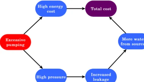
The method involves utilisation of a hydraulic model of the network with pressure dependent leakage and inclusion of a simplified PRV model with the PRV set-points included in a set of decision variables. The cost function represents the total cost of water treatment and pumping. Figure 1 illustrates that with such approach an excessive pumping contributes to a high total cost in two ways. Firstly, it leads to high energy usage. Secondly, it induces high pressure, hence increased leakage, which means that more water needs to be pumped and taken from sources. Therefore, the optimizer attempts to reduce both energy usage and leakage by minimising the total cost.
Figure 1.Illustrating how excessive pumping contributes to high total cost when network model with pressure dependent leakage is used.
Details about the model reduction algorithm are given in Paluszczyszyn et al. (2013) and Alzamora et al. (2014).
Some decision variables of the considered optimisation problem are continuous (e.g. water production, pump speed, valve opening) and some are integer (e.g. number of pumps switched on). Problems containing both continuous and inte-ger variables are called mixed-inteinte-ger problems and are hard to solve numerically, particularly when the problem is also non-linear. Continuous relaxation of integer variables (e.g. allowing 2.5 pumps switched on) enables network schedul-ing to be treated initially as a continuous optimisation prob-lem solved by a non-linear programming algorithm. Subse-quently, the continuous solution can be transformed into an integer solution by manual post-processing, or by further op-timisation. For example, the result “2.5 pumps switched on” can be realised by a combination of 2 and 3 pumps switched over the time step. Note that an experienced network oper-ator is able to manually transform continuous pump sched-ules into equivalent discrete schedsched-ules. In this work the main focus is on obtaining the continuous schedules; however, two simple schedules discretisation approaches are also pre-sented in Sect. 4, one fully-automatic and one interactive.
2.2 Implementation
The main software module has been implemented in C# and .NET 4.0. Using a simplified hydraulic model of network in the EPANET format and additional files the optimisa-tion problem is automatically generated by the main software module in a mathematical modelling language called GAMS (Brooke et al., 1998). Subsequently, a non-linear program-ming solver called CONOPT is called to calculate a contin-uous optimisation solution. An optimal solution is then fed back from CONOPT into the main software module for anal-ysis and/or further processing and/or export of the results. Specific details of the software functions are as follows:
1. Loads input files required to formulate the optimisation problem (details are given below).
2. Validates the model, i.e. ensures that e.g.: no control rules are associated with pumps or pipes, pressure at leakage nodes is positive, tanks are not emptying or overflowing.
3. Generates GAMS code, runs GAMS (which calls CONOPT), retrieves GAMS results.
4. Handles manipulation of the EPANET model which is required to: (i) use initial schedules (if required) from external time-series files, (ii) manipulate schedules for the purpose of interactive discretisation described in Sect. 4, (iii) produce EPANET file with optimal pump and valve schedules. Note that due to EPANET limita-tions (Rossman, 2000) valve schedules are implemented as time-based control rules.
5. Handles manipulation of xls files for the purpose of in-teractive discretisation.
6. Produces time-series files with optimal pump and valve schedules and the resulting tank level trajectories.
Complete information of the WDN and other data required to formulate the optimisation problem is obtained from the following sources:
1. EPANET input file (inp format),
2. EPANET binary simulation results file (bin format) pro-duced by calling the simulator,
3. time-series files (csv format) describing initial sched-ules; when the scheduler is employed in an on-line receding-horizon environment (Skworcow et al., 2010), the schedules from the previous time step can be used as an initial condition for the current time step,
4. electricity tariffs (csv format),
5. configuration files (txt format) describing the following:
– lengths of time step and optimisation horizon, – configuration of pump stations: (i) fixed or
vari-able speed, (ii) which pump in EPANET belongs to which pump station, (iii) hydraulic curve and power curve coefficients, (iv) constraints: min. and max. number of pumps switched on, min. and max. speed, max. flow,
– min. and max. flow in pipes and valves, – min. and max. pressure at connection nodes, – tank level constraints (which are not
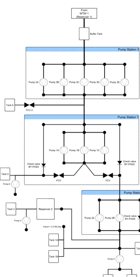
Figure 2.A schematic of the network.
3 Water distribution network scheduling: continuous optimisation
In this section details on formulating and solving a con-tinuous optimisation problem are given. Initial conditions for all variables (flows, pressures etc.) are obtained directly from the EPANET output file from which the network struc-ture was loaded. The optimisation problem has the following three elements, which are described in details in the follow-ing subsections: (i) hydraulic model of the network, (ii) ob-jective function, (iii) constraints. The problem is expressed in discrete time withkdenoting time step.
3.1 Modelling of WDN for optimisation in GAMS
Each network component has a hydraulic equation. Tanks and pump stations are represented by standard models see e.g. Brdys and Ulanicki (1994) and pipes are represented by the Hazen–Williams formula. A pump station model requires also an additional hydraulic equation and an electrical power characteristic equation. For valves simplified equations are used; details concerning pumps and valves modelling are given below.
3.1.1 Connection nodes
For connection nodes, mass-balance equation is employed; however, since leakage is assumed to be at connection nodes, the standard mass balance equation is modified to include the leakage term:
3cq(k)+dc(k)+lc(k)=0 (1)
where3cis a node branch incidence matrix,qis a vector of
branch flows,dcdenotes a vector of demands andlcdenotes
a vector of leakages calculated as:
lc(k)=pα(k)κ (2)
with p denoting a vector of node pressures, α denoting a leakage exponent andκ denoting a vector of leakage co-efficients, see Ulanicki et al. (2000) for details. Note that in the GAMS implementation the variables describing pressure at nodes with non-zero leakage coefficientκ are constrained to be positive, whilst the leakage term in Eq. (1) is zero for nodes with zero leakage coefficientκ.
3.1.2 Pump stations
It is assumed that all pumps in any pump station have the same characteristics as in Brdys and Ulanicki (1994). In ad-dition to the standard hydraulic equation which forces the pump station to operate along its head-flow curve the follow-ing equation for each pump station is added:
1h(k)u(k)≥0 (3)
where1hdenotes head increase between inlet and outlet and
udenotes number of pumps switched on.
station and a negative head increase on the upstream pump station, such that the total head increase (from both pump stations) would still satisfy other constraints and equations. Consequently, Eq. (3) is required for networks with pump stations connected in series to ensure physical feasibility of the solution.
To model electricity usage, instead of using a pump effi-ciency equation a direct modelling of pump station power is employed, as discussed in Ulanicki et al. (2008). However, the equation is rearranged to allow zero pumps switched on, without introducing if-else formulas:
P (k)u(k)2=Eq(k)3+F q(k)2u(k)s(k)+
Gq(k)u(k)2s(k)2+H u(k)3s(k)3 (4)
whereE, F, G, H are power coefficients constant for a given pump station, q is flow,P is consumed power, s is speed normalised to a nominal speed for which the pump hydraulic curve was obtained. Additionally it is imposed for all pump stations thatP (k)≥0, so when all pumps in a given pump station are switched off (i.e.u(k)=0) the solver (due to min-imising the cost) assignsP (k)=0 for this pump station. Fi-nally, since the coefficientsEandF are small compared to
G andH, to make a large-scale model easier to solve it is assumed thatE=0 andF=0, i.e. the consumed power de-pends linearly on the pump station flow.
3.1.3 Valves
There are different types of valves in WDN that can be con-trolled remotely and/or according to a time-schedule; for some, valve opening is controlled directly, while for others pressure drop or flow across the valve is controlled. In the approach proposed in this paper all controllable valves are assumed to be PRVs (control variable is PRV outlet pressure) or FCV (control variable is valve flow). Actual implementa-tion of the control variables in the physical WDN depends on valve construction and is not considered here.
Since head-loss across the valve can be regulated for both FCV and PRV and their direction of flow is known, to reduce the nonlinearity of the model it is proposed to express both FCV and PRV as two simple inequalities:
hin(k) > hout(k) q(k)≥0 (5)
with the difference between both valve types being their con-trol variables: flow for FCV and outlet pressure for PRV. Consequently, valve flow is defined by other network ele-ments and the mass-balance equation.
Check-valves (non-return valves) are described by the fol-lowing equation:
q(k)=max
0,|1h(k)|
R0.54 sign(1h(k))
(6)
whereRis a constant valve resistance. Such formulation en-sures that valve head-loss is positive if and only if valve flow
is greater than zero; when the flow is zero (i.e. check valve is closed) the head-loss can take any negative value, i.e. inlet and outlet pressures are defined by other network elements. Note that in the Hazen–Williams formula|1h|0.54 is used, while here to reduce the nonlinearity of the model it is pro-posed to use|1h|. The justification for such simplification is that head-loss across an open check-valve is relatively small compared to head-loss in other elements, hence such simpli-fication has negligible effects on obtained results. To avoid unnecessary discontinuities, the term sign(1h)in Eq. (6) is actually implemented as:
sign(1h)≈ 1h
|1h| +10−14 (7)
3.2 Objective function
The objective function to be minimised is the total energy cost for water treatment and pumping. Pumping cost depends on the consumed power and the electricity tariff over the pumping duration. The tariff is usually a function of time with cheaper and more expensive periods. For given time step
τc, the objective function considered over a given time
hori-zon
k0, kfis described by the following equation:
φ=
X
j∈Jp
kf
X
k=k0
γpj(k)Pj(k)+
X
j∈Js
kf
X
k=k0
γsj(k)qsj(k)
τc (8)
hereJpis the set of indices for pump stations andJs is the
set of indices for treatment works. The functionγpj(k)
repre-sents the electricity tariff. The treatment cost for each treat-ment works is proportional to the flow output with the time-dependent unit price of γsj(k). The term Pj represents the
electrical power consumed by pump stationj and is calcu-lated according to Eq. (4).
3.3 Operational constraints
In addition to constraints described by the hydraulic model equations defined above, operational constraints are applied to keep the system-state within its feasible range. Practical requirements are translated from the linguistic statements into mathematical inequalities. The typical requirements of network scheduling are concerned with tank levels in order to prevent emptying or overflowing, and to maintain adequate storage for emergency purposes:
hmin(k)≤h(k)≤hmax(k) for k∈k0, kf (9)
The control variables such as the number of pumps switched on in each pump station, pump speeds or valve flow, are also constrained by lower and upper constraints determined by the features of the control components.
It is evident from the above equations that the overall opti-misation model is nonlinear. Furthermore, GAMS recognizes that the model is non-smooth due to the term|1h|in Eq. (7). Hence, the overall optimisation model is of the form Nonlin-ear Programming with Discontinuous Derivatives (DNLP).
4 Discretisation of continuous schedules
The main focus of this paper is on the continuous opti-misation, hence only two simple discretisation approaches are discussed: (i) a fully-automatic discretisation algorithm which does not rely on the EPANET simulation engine but uses GAMS and simple heuristics, and (ii) an interactive dis-cretisation which uses EPANET simulation engine. Both ap-proaches assume that the discretisation time step length is shorter than the continuous optimisation time step length, so for example continuous “2.5 pump switched on for 2 h”, can be discretised as “3 pumps on for 1 h and then 2 pumps on for another hour”.
4.1 Automatic discretisation
The algorithms progresses through the following steps:
1. Load continuous optimisation results produced by GAMS/CONOPT.
2. For each pump station round the continuous pump con-trol (i.e. the number of pumps switched on) to an integer number, while calculating an accumulated rounding er-ror at each time step. The accumulated rounding erer-ror is used at subsequent time steps to decide whether the number of pumps switched on should be rounded up or down, using user-defined thresholds.
3. Generate a new GAMS code where the number of pumps switched on for each pump station and at each time step are fixed, i.e. as calculated in step 2. Initial conditions for all flows and pressures in the network are as calculated by GAMS/CONOPT during the con-tinuous optimisation. Note that in this GAMS code the number of pumps switched on for each pump station and at each time step are no longer decision variables but forced parameters. However, the solver (CONOPT) can still change pump speed and can adjust valve flow to match the integer number of pumps switched on. The cost function to be minimised and the constraints are the same as in the continuous optimisation.
4. Call GAMS/CONOPT and subsequently load the re-sults of integer optimised solution.
5. During the continuous optimisation, pump station flow can be zero only when all pumps in this station are off. However, in the integer optimisation over a long time horizon it may happen that pump station control is forced to have e.g. 1 pump switched on during a par-ticular time step, but this pump is unable to deliver the required head at that time step, hence the pump flow is zero. If such event occurs, the above steps 3 and 4 are repeated, but at the time steps when the resulting pump station flow was zero, the number of pumps switched on is forced to be zero.
4.2 Interactive discretisation
The interactive discretisation approach involves the use of the EPANET simulation engine and a spreadsheet software. The role of the user is to manipulate the discrete schedules initially proposed by the scheduler, by modifying at which time steps the number of pumps switched on is rounded up or down. For networks with flow control valves (FCV) diverting the flow from one pump station into multiple branches, the user may also need to modify the FCV control to match the modified discrete pump schedule. For example, if the con-tinuous pump control at a particular time step is 2.5 pump switched on for 2 h, and it is discretised as 3 pumps on for 1 h and then 2 pumps on for another hour, then the required FCV flow which was calculated during the continuous opti-misation needs to be modified to account for increased flow during the first hour and decreased flow during the second hour. The interactive discretisation process progresses itera-tively through the following steps, note that the points 1 and 2 in both automatic and interactive discretisation are the same:
1. Load continuous optimisation results produced by GAMS/CONOPT.
2. For each pump station round the continuous pump con-trol (i.e. the number of pumps switched on) to an integer number, thus generating initial discrete schedules.
3. Automatically update the EPANET model with new dis-crete schedules, simulate the model and retrieve the hy-draulic results.
4. Automatically generate an xls file with continuous and discrete schedules, hydraulic results and costs. The file also contains tariffs, plots and other features to simplify the analysis and schedules manipulation.
6. Automatically load the updated discrete schedules from the xls file into the scheduler and go to point 3. The pro-cess described in points 3–6 is repeated until the user decides that the results obtained from the discrete sched-ules and from the continuous optimisation are suffi-ciently close. For small networks or a short time horizon (24 h) only few iterations are required. For large, com-plex networks and a long time horizon (7 days) more than ten iterations may be required.
5 Case study: large-scale WDN
This section describes application of the proposed method to optimise operation of a large-scale WDN. The study was based on real data concerning an actual WDN being part of a major water company in the UK.
5.1 Network overview
The considered WDN consists of 12 363 nodes, 12 923 pipes, 4 (forced-head) reservoirs, 10 (variable-head) tanks, 13 pumps in 6 pump stations and 315 valves. The average demand is 451 L s−1(39 ML day−1). The system is supplied from 1 major source (water-treatment works) and 2 small imports (under 0.2 ML day−1). The model was provided in the EPANET format. The considered WDN includes com-plex structures and interactions between pump stations, e.g. pump stations in series without an intermediate tank, pump stations with by-passes, mixture of fixed-speed and variable-speed pump stations, valves diverting the flow from one pump station into many tanks, PRVs fed from booster pumps or a booster pump fed from a PRV.
Due to the network complexity only its schematic with configuration of pump stations is illustrated in Fig. 2. Due to pump station by-passes, when the demand between two pump stations connected in series is low (i.e. at night), one of the pump stations can be turned off and the water will still reach the downstream part of the network with a sufficient pressure.
5.2 Hydraulic model preparation and simplification Before the automatic model reduction algorithm was applied some manual model preparation was carried out; this in-cluded:
1. The model was converted from the Darcy–Weisbach formula to the Hazen–Williams formula, using an op-erating point when most of the pumps were switched on, i.e. when the flow in pipes was high.
2. Two reservoirs were connected to the system via perma-nently closed pipelines; these reservoirs were removed.
3. Two connected tanks that follow a similar pressure tra-jectory were merged into one tank with a suitably cho-sen diameter.
4. Around 200 permanently closed isolation valves were removed.
5. Several valves that had fixed opening (i.e. throttle con-trol valves (TCV) without any concon-trol rules assigned) were replaced with pipes of an equivalent resistance.
6. A TCV to which an open-close control rule was as-signed was replaced with an equivalent FCV.
7. A pipe to which an open-close control rule was assigned was replaced with an equivalent valve (FCV) to ensure that only control elements are actually controlled in the model.
The above modifications enable further reduction in the number of network elements; for example, if the isolation valves were not removed, the automatic model reduction al-gorithm would treat them as control elements, thus retain-ing them in the reduced model. Table 1 presents functions of valves in the original model and actions performed during the model reduction. Subsequently, the automatic model reduc-tion algorithm was applied; the scale of reducreduc-tion is shown in Table 2. The model reduction algorithm requires an op-erating point around which the model will be linearised; in such complex WDN selection of the operating point might present a challenge. However, keeping in mind that the oper-ating point should be representative for normal operation of the network and should be chosen for average demand con-ditions while keeping at least one pumping unit working at each pumping station (Alzamora et al., 2014), the operating point was chosen at 12:30 h.
To validate how the reduced model replicates the hydraulic behaviour of the original model a goodness of fit in terms of
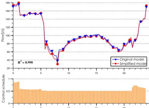
R2was calculated for flow trajectories of pumps/valves and for head trajectories of reservoirs/tanks. It was found that the reduced model adequately replicates the hydraulic behaviour of the original model. TheR2for pump and valve flows was 0.94 in the worst case, 0.99 for most cases and 1.0 for some elements. The R2 for reservoirs and tanks was 0.5 in the worst case, 0.91 in the second-to-worst case, and between 0.98 and 1.0 for all other reservoirs and tanks. The largest discrepancy was at a small tank which was the furthest from the main source and was empty (according to the original model) at around 18:00 h. Typical performance (i.e. with ac-curacy obtained for most elements) of the reduced model is illustrated in Figs. 3 and 4. Detailed analysis revealed that the most significant errors were introduced due to the conversion from the Darcy–Weisbach formula to the Hazen–Williams formula.
5.3 Example scheduling results and discussion
Table 1.Function of each valve in the original model and actions performed during the model reduction.(∗)not classified as a valve in the total valves count in the original model.
Type Status # in Action # in
original model reduced model
PRV permanently closed 3 removed 0
active 39 retained 39
FCV active 1 retained 1
TCV close-open control rule 1 converted to FCV 0 (1)
isolation valve 51 removed 0
constant opening 220 converted to pipe 0
Pipe∗ close-open control rule 1 converted to FCV 0 (1)
Total 315 39 (42)
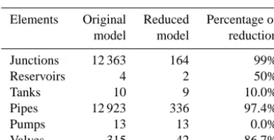
Table 2.Number of elements in the original and the reduced model.
Elements Original Reduced Percentage of model model reduction
Junctions 12 363 164 99%
Reservoirs 4 2 50%
Tanks 10 9 10.0%
Pipes 12 923 336 97.4%
Pumps 13 13 0.0%
Valves 315 42 86.7%
horizons (24 h and 7 days), with/without pressure dependent leakage and with different demand levels (scaled for differ-ent seasons). In all considered scenarios the initial tank level for each tank was assumed to be as in the provided EPANET model. Pressure and flow constraints in different elements were either provided by the water company or assumed and were kept constant for all scenarios. In each case a GAMS code was automatically generated and CONOPT managed to find an optimal continuous solution. However, the automatic discretisation required several trials with different thresholds mentioned in Sect. 4.1. The automatic discretisation algo-rithm particularly struggled for scenarios with pressure de-pendent leakage; for these scenarios the interactive discreti-sation approach was employed.
Subsequently, it was decided to extend the boundaries of the model and include an additional pump station and a tank. After the changes were made in the simplified EPANET model and in an additional file describing pump station con-straints, the scheduler successfully generated and solved an updated optimisation model without the need of any changes to the algorithm. Optimisation for 24 h horizon with 1 h time-step and for 7 days horizon with 2 h time-time-step took around 5 min and 1 h, respectively, on a standard office PC.
It was observed that for all 24 h horizon scenarios it was not possible to fully utilise the allowed capacity of the large tanks and their levels were far from the allowed limits. This was due to the restriction that the final tank level must be
0 5 10 15 20 25
101 101.1 101.2 101.3 101.4 101.5 101.6
H
e
a
d
[
m]
Time [h]
0 5 10 15 20 25
−40 −20 0 20 40 60 80
F
lo
w
[
l/s
]
Original in-out flow Reduced in-out flow Tank flow disparity Original tank trajectory Reduced tank trajectory
Mass balance error = 0.062 [Ml/day] R2 = 0.993
Relative error = 0.538 [%]
Figure 3.Typical discrepancy in tank level in the original and sim-plified models.
P. Skworcow et al.: Pump schedules optimisation 61
0 5 10 15 20 25
20 40 60 80 100 120 140 160 180 F lo w [l /s ] Original model Simplified model
0 5 10 15 20 25
0 0.5 1 Co n tr o l s ch e d u le Time [h] R2 = 0.990
Figure 4.Typical discrepancy in performance of a pump station in the original and simplified models.
els were far from the initial ones for most tanks. However, the costs for different scenarios were compared against each other. This allowed to formulate several conclusions useful for the water company. For example, two scenarios named A and B considered identical constraints, demands, leakage and topology, but in scenario A a pump station in the mid-dle of the network was fixed speed (as is at present in the physical system) and in scenario B this pump station was equipped with variable speed drive, with the hydraulic and power curves for this pump station being identical in both scenarios A and B. It was found that in scenario B the pump station still operated at 100 % speed for majority of time, even when the initial condition was given as 70 %, and the reduction in cost was minimal compared to scenario A. Thus actual installation of a variable speed drive in this pump sta-tion in the physical system would not reduce the pumping cost; this demonstrates how the proposed approach can be used to evaluate cost-effectiveness of potential investment in assets related to pumping.
Figure 5.An example schedule for the largest pump station.
0 12 23 45 36 50 72 63 85 106 120 142 133 195 156 2 29 4 49 3 2 !"#"!
Figure 6.An example tank level trajectory.
6 Conclusions
Pump operation optimisation is a difficult task due to sig-nificant complexity and inherent non-linearity of WDNs. In this paper a time-schedules optimisation is considered and simultaneous optimisation of pumps and valves schedules is employed. An optimisation model is automatically generated in the GAMS language from a hydraulic model in EPANET format and from additional files describing operational con-straints, electricity tariffs and pump station configurations. In order to reduce the size of the optimisation problem the full hydraulic model is simplified using a model reduction al-gorithm. A nonlinear programming solver CONOPT is used to solve the continuous optimisation problem. Subsequently, the schedules are converted to a mixed-integer form using a simple heuristic.
The proposed approached was tested on a large-scale WDN being part of a major UK water company and pro-vided in EPANET format. The considered WDN included complex structures and interactions between pump stations. Solving of several scenarios considering different horizons, time steps and operational constraints, and also with topo-logical changes to the hydraulic model demonstrated ability of the approach to automatically generate and solve optimi-sation problems for a variety of requirements. However, fur-ther work is required to improve the current discretisation approaches.
References
Abdelmeguid, H. and Ulanicki, B.: Feedback rules for operation of pumps in a water supply system considering electricity tariffs, in: Water Distribution Systems Analysis, 1188–1205, 2010. Alzamora, F., Ulanicki, B., and Salomons, E.: A Fast and Practical
Method for Model Reduction of Large Scale Water Distribution Networks, J. Water Res. Pl.-ASCE, 140, 444–456, 2014. Bentley Systems: Darwin Scheduler, http://www.bentley.com/
en-GB/Products/WaterCAD/Darwin-Scheduler.htm/, last access: 17 April 2014.
Brdys, M. and Ulanicki, B.: Water Systems: Structures, Algorithms and Applications, Prentice Hall, UK, 1994.
Brooke, A., Kendrick, D., Meeraus, A., and Raman, R.: GAMS: A user’s guide, GAMS Development Corporation, Washington, DC, USA, 1998.
Bunn, S. and Reynolds, L.: The energy-efficiency benefits of pump-scheduling optimization for potable water supplies, IBM J. Res. Dev., 53, 5:1–5:13, 2009.
Derceto Inc.: Derceto Aquadapt, http://www.derceto.com/ Products-Services/Derceto-Aquadapt/, last access: 17 April 2014.
Farmani, R., Walters, G., and Savic, D.: Evolutionary multi-objective optimization of the design and operation of water dis-tribution network – total cost vs reliability vs water quality, J. Hydroinform., 8, 165–179, 2006.
Fiorelli, D., Schutz, G., Metla, N., and Meyers, J.: Appli-cation of an optimal predictive controller for a small wa-Figure 5.An example schedule for the largest pump station.
optimisation point of view. Therefore, maximising the level in that particular tank enabled small reduction in pumping effort on the downstream pumping station.
Note that the current and optimised operations are not compared, since the provided data considered only one day of operation and on that particular day the final tank lev-els were far from the initial ones for most tanks. However, the costs for different scenarios were compared against each other. This allowed to formulate several conclusions useful for the water company. For example, two scenarios named A and B considered identical constraints, demands, leakage and topology, but in scenario A a pump station in the mid-dle of the network was fixed speed (as is at present in the physical system) and in scenario B this pump station was equipped with variable speed drive, with the hydraulic and power curves for this pump station being identical in both scenarios A and B. It was found that in scenario B the pump
0 12 23 45 36 50 72 63 85 106 120 142 133 195 156 2 29 4 49 3 2 !"#"!
Figure 6.An example tank level trajectory.
station still operated at 100 % speed for majority of time, even when the initial condition was given as 70 %, and the reduction in cost was minimal compared to scenario A. Thus actual installation of a variable speed drive in this pump sta-tion in the physical system would not reduce the pumping cost; this demonstrates how the proposed approach can be used to evaluate cost-effectiveness of potential investment in assets related to pumping.
6 Conclusions
Pump operation optimisation is a difficult task due to signifi-cant complexity and inherent non-linearity of WDNs. In this paper a time-schedules optimisation is considered and simul-taneous optimisation of pumps and valves schedules is em-ployed. An optimisation model is automatically generated in the GAMS language from a hydraulic model in the EPANET format and from additional files describing operational con-straints, electricity tariffs and pump station configurations. In order to reduce the size of the optimisation problem the full hydraulic model is simplified using a model reduction al-gorithm. A nonlinear programming solver CONOPT is used to solve the continuous optimisation problem. Subsequently, the schedules are converted to a mixed-integer form using a simple heuristic.
The proposed approached was tested on a large-scale WDN being part of a major UK water company and provided in the EPANET format. The considered WDN included complex structures and interactions between pump stations. Solving of several scenarios considering different horizons, time steps and operational constraints, and also with topological changes to the hydraulic model demon-strated ability of the approach to automatically generate and solve optimisation problems for a variety of requirements. However, further work is required to improve the current discretisation approaches.
References
Abdelmeguid, H. and Ulanicki, B.: Feedback rules for operation of pumps in a water supply system considering electricity tariffs, in: Water Distribution Systems Analysis, 1188–1205, 2010. Alzamora, F., Ulanicki, B., and Salomons, E.: A Fast and Practical
Method for Model Reduction of Large Scale Water Distribution Networks, J. Water Res. Pl.-ASCE, 140, 444–456, 2014. Bentley Systems: Darwin Scheduler, http://www.bentley.com/
en-GB/Products/WaterCAD/Darwin-Scheduler.htm/, last ac-cess: 17 April 2014.
Brdys, M. and Ulanicki, B.: Water Systems: Structures, Algorithms and Applications, Prentice Hall, UK, 1994.
Brooke, A., Kendrick, D., Meeraus, A., and Raman, R.: GAMS: A user’s guide, GAMS Development Corporation, Washington, DC, USA, 1998.
Bunn, S. and Reynolds, L.: The energy-efficiency benefits of pump-scheduling optimization for potable water supplies, IBM J. Res. Dev., 53, 5:1–5:13, 2009.
Derceto Inc.: Derceto Aquadapt, http://www.derceto.com/ Products-Services/Derceto-Aquadapt/, last access: 17 April 2014.
Farmani, R., Walters, G., and Savic, D.: Evolutionary multi-objective optimization of the design and operation of water dis-tribution network – total cost vs reliability vs water quality, J. Hydroinform., 8, 165–179, 2006.
Fiorelli, D., Schutz, G., Metla, N., and Meyers, J.: Application of an optimal predictive controller for a small water distribution net-work in Luxembourg, J. Hydroinform., 15, 625–633, 2012. Geem, Z.: Harmony search optimisation to the pump-included
wa-ter distribution network design, Civil Eng. Environ. Syst., 26, 211–221, 2009.
Innovyze: BalanceNet, http://www.innovyze.com/products/ balancenet/, last access: 30 December 2013.
Lopez-Ibanez, M., Prasad, T., and Paechter, B.: Ant colony opti-mization for optimal control of pumps in water distribution net-works, J. Water Res. Pl-ASCE, 134, 337–346, 2008.
McCormick, G. and Powell, R.: Optimal Pump Scheduling in Water Supply Systems with Maximum Demand Charges, J. Water Res. Pl.-ASCE, 129, 372–379, 2003.
Paluszczyszyn, D., Skworcow, P., and Ulanicki, B.: Online simplifi-cation of water distribution network models for optimal schedul-ing, J. Hydroinform., 15, 652–665, 2013.
Price, E. and Ostfeld, A.: Iterative Linearization Scheme for Convex Nonlinear Equations: Application to Optimal Operation of Wa-ter Distribution Systems, J. WaWa-ter Res. Pl.-ASCE, 139, 299–312, 2013.
Rossman, L.: EPANET Users manual, US: Risk Reduction Engi-neering Laboratory, Office of Research and Development, US Enviromental Protection Agency, Cincinnati, Ohio, USA, 2000. Salomons, E., Goryashko, A., Shamir, U., Rao, Z., and Alvisi, S.:
Optimizing the operation of the Haifa-A water-distribution net-work, J. Hydroinform., 9, 51–64, 2007.
Skworcow, P., AbdelMeguid, H., Ulanicki, B., and Bounds, P.: Op-timal pump scheduling with pressure control aspects: Case stud-ies, in: Integrating Water Systems: Proceedings of the 10th In-ternational Conference on Computing and Control in the Water Industry, 2009a.
Skworcow, P., AbdelMeguid, H., Ulanicki, B., Bounds, P., and Pa-tel, R.: Combined energy and pressure management in water dis-tribution systems, in: 11th Water Disdis-tribution Systems Analysis Symposium, Kansas City, USA, 2009b.
Skworcow, P., Ulanicki, B., AbdelMeguid, H., and Paluszczyszyn, D.: Model predictive control for energy and leakage management in water distribution systems, in: UKACC International Conference on Control, Coventry, UK, 2010.
Ulanicki, B., Bounds, P., Rance, J., and Reynolds, L.: Open and closed loop pressure control for leakage reduction, Urban Water J., 2, 105–114, 2000.
Ulanicki, B., Kahler, J., and See, H.: Dynamic optimization ap-proach for solving an optimal scheduling problem in water dis-tribution systems, J. Water Res. Pl.-ASCE, 133, 23–32, 2007. Ulanicki, B., Kahler, J., and Coulbeck, B.: Modeling the efficiency