https://doi.org/10.5194/se-8-969-2017
© Author(s) 2017. This work is distributed under the Creative Commons Attribution 3.0 License.
Element-by-element parallel spectral-element methods for 3-D
teleseismic wave modeling
Shaolin Liu1, Dinghui Yang1, Xingpeng Dong1, Qiancheng Liu2, and Yongchang Zheng3 1Department of Mathematical Sciences, Tsinghua University, Beijing, 100084, China
2King Abdullah University of Science and Technology, Thuwal 23955-6900, Saudi Arabia
3Department of Liver Surgery, Peking Union Medical College Hospital, Chinese Academy of Medical Sciences and Peking Union Medical College, Beijing, 100730, China
Correspondence to:Dinghui Yang ([email protected]) Received: 14 April 2017 – Discussion started: 8 May 2017
Revised: 17 August 2017 – Accepted: 30 August 2017 – Published: 28 September 2017
Abstract.The development of an efficient algorithm for tele-seismic wave field modeling is valuable for calculating the gradients of the misfit function (termed “misfit gradients”) or Fréchet derivatives when the teleseismic waveform is used for adjoint tomography. Here, we introduce an element-by-element parallel spectral-element-by-element method (EBE-SEM) for the efficient modeling of teleseismic wave field propagation in a reduced geology model. Under the plane-wave assump-tion, the frequency–wavenumber (FK) technique is imple-mented to compute the boundary wave field used to con-struct the boundary condition of the teleseismic wave inci-dence. To reduce the memory required for the storage of the boundary wave field for the incidence boundary condition, a strategy is introduced to efficiently store the boundary wave field on the model boundary. The perfectly matched layers absorbing boundary condition (PML ABC) is formulated us-ing the EBE-SEM to absorb the scattered wave field from the model interior. The misfit gradient can easily be constructed in each time step during the calculation of the adjoint wave field. Three synthetic examples demonstrate the validity of the EBE-SEM for use in teleseismic wave field modeling and the misfit gradient calculation.
1 Introduction
The increasing demand for high-resolution imaging of deep lithospheric structures requires the utilization of teleseis-mic datasets for waveform inversion. Teleseisteleseis-mic waves pro-vide tremendous amounts of information for the detection of
crustal and upper mantle structures (Rondenay, 2009). Over the past forty years, many techniques have been developed to analyze teleseismic wave datasets, including receiver func-tion analysis (Langston, 1977; Kind et al., 2012), teleseismic wave travel-time tomography based on ray theory (Zhang et al., 2011), teleseismic migration (Shragge et al., 2006), and teleseismic scattering tomography (Roecker et al., 2010; Tong et al., 2014a). To achieve the high-resolution imag-ing of lithospheric structures, the adjoint-state method has become the state-of-the-art technique for teleseismic wave imaging (Tong et al., 2014a; Monteiller et al., 2015).
full-wave field simulations are required to perform an adjoint tomography inversion (Tape et al., 2007, 2009).
Because most earthquakes occur in the crust, and seismic rays cannot easily illuminate the deep lithosphere in local seismic tomography, imaging the deep lithospheric structures can be difficult (Tong et al., 2014b, c). Increasing the model size enables more deep reflections and refractions to be in-cluded in the inversion dataset; as a result, deep structures can be inverted by fitting these reflected and refracted wave-forms (Chen et al., 2015). However, for continental-scale models, it is difficult to invert short-period seismic data on a standard computing cluster, such as 1–2 s for P waves and 3–6 s for S waves (Tong et al., 2015).
To reduce the amount of computation involved in solving the full seismic wave equation, many hybrid methods have been developed to localize 2-D/3-D numerical solvers. The boundary conditions for the reduced simulation model are provided by rapid 1-D analytical solutions for the 1-D back-ground Earth model (Capdeville et al., 2003; Monteiller et al., 2013, 2015; Tong et al., 2014a, 2015). The 2-D/3-D re-sponses to the heterogeneity inside the reduced model con-tribute to the coda waves of the teleseismic phases, and the 2-D/3-D effects outside the model are neglected. This assump-tion of a 1-D background layered Earth model is similar to that in receiver function analysis and is often effective for a station that is sufficiently far from the source (Langston, 1977; Rondenay, 2009).
Although the computational requirements can be effi-ciently reduced by these hybrid methods, the computational costs are still excessive for a small workstation when we are faced with the several thousand forward simulations required in 3-D teleseismic adjoint tomography. To further reduce the computational costs, Roecker et al. (2010) constructed a fre-quency domain 2.5-D hybrid method for teleseismic wave simulations. To simplify the teleseismic wave field invari-ant along a particular axis, the 2.5-D formulation can sig-nificantly reduce the computational demands. However, the 2.5-D formulation may restrict the application of the method in arbitrarily heterogeneous media (Tong et al., 2015).
In addition to the large computational demand (CPU time) associated with the 3-D hybrid methods, satisfying the mem-ory requirements for storing the boundary wave fields to con-struct teleseismic incident boundary conditions is another important issue that should be carefully considered. Tong et al. (2015) adapted the Clayton and Engquist-type (CE-type) boundary condition (Clayton and Engquist, 1977) to inter-face the 1-D background analytical solution with a numerical solver on the boundary of a reduced model. This treatment can both assign the teleseismic incident condition for the computational domain and absorb the scattered wave field from the interior of the heterogeneous model. Implement-ing the CE-type boundary condition is extremely simple and does not substantially increase the required CPU time. How-ever, the CE-type boundary condition can efficiently absorb waves only at approximately normal incident angles, and
in-cident waves at grazing angles may be reflected back to the model (Yang et al., 2003), which may reduce the accuracy of the forward and adjoint wave fields in teleseismic adjoint to-mography and thus decrease the accuracy of the constructed Fréchet derivatives. Note that the CE-type boundary condi-tion requires nine wave field components (three displace-ment components and six stress components) to be stored on the model boundary; this requirement may be a significant burden on the computer memory for a relatively large-scale model decomposed by a dense numerical mesh.
Here, we introduce the element-by-element parallel spectral-element method (EBE-SEM) for the efficient eling of teleseismic plane-wave propagation in reduced mod-els. A significant advantage of the EBE-SEM is the easy par-allelization of the spectral-element algorithm, which does not require the assembly of the global stiffness matrix. The spec-tral elements are equally allocated to every CPU core, and the product of the stiffness matrix and the solution vector is calculated element by element; these aspects are quite useful for ensuring load balance among the CPU cores. The ele-ment stiffness matrix can be written as the tensor product of the submatrices, which greatly reduce the computer memory. In addition, the misfit gradient can be efficiently constructed because the element matrices for calculating the misfit gra-dient can also be formulated from the tensor products of the element submatrices. The perfectly matched layers (PMLs; Collino and Tsogka, 2001; Komatitsch and Tromp, 2003; Liu et al., 2014) are formulated by the EBE-SEM to effectively absorb scattered waves. A detailed discussion is presented to incorporate the teleseismic incident boundary condition in the EBE-SEM, and only six components on the interface be-tween the computational domain and the PML domain must be stored in the computer memory. The high efficiency of the EBE-SEM for teleseismic wave modeling and misfit gra-dient construction is demonstrated by using three numerical examples.
2 EBE-SEM
q
x
y
z
Crust
Mantle A
Figure 1.Schematic of a teleseismic plane wave entering a local two-layered crust–upper-mantle model. The study area is delineated by the blue lines. The origin of the Cartesian system is located on the surface at corner A of the model. The positivexandydirections point to the east and south, respectively, and the positivez direc-tion points downward. The inverted red triangle located at (60 km, 60 km, 0 km) represents a seismic station. The plane in the lower left of the figure denotes the wave front of the incident teleseismic plane wave. The purple arrows indicates the normal vector of the plane wave. The incident angle isθ, which is the angle between the normal vector and –z. The azimuth angle isϕ, which is the angle between the projection of the normal vector into thex–yplane and –y. The azimuth angle is not explicitly shown in this figure.
2.1 EBE-SEM for total wave simulation
We assume that the total wave field obeys the following elas-tic wave equation (Tong et al., 2014a):
ρu¨t= ∇ · h
λ (∇ ·ut)I+µ
∇ut+ ∇uTt i
, (1)
where the two dots above ut denote the second-order time derivative,Iis the 3×3 identity matrix,λandµare Lamé pa-rameters,∇ = ex∂x+ey∂y+ez∂zis the gradient operator,
and the superscriptT denotes the matrix transpose operation. Following the classical SEM (Seriani, 1997; Komatitsch and Vilotte, 1998; Komatitsch and Tromp, 2002), using an arbi-trary test vector v to multiply both sides of Eq. (1) and in-tegrating over the domain, we obtain the following weak
form wave equation: Z
v· ¨utd+ Z
∇v:λ (∇ ·ut)I+µ
∇ut+ ∇uTt
d
=
Z
∂
v·σt·nds, (2)
wherenis the normal vector of the boundary∂. The defini-tion of the double dot product can be found in De Basabe and Sen (2007). Under the natural boundary condition, the right side of Eq. (2) is 0. If the infinite space is decomposed into
N nonoverlapping hexahedral elements, then Eq. (2) can be written as
N
X
e=1 Z
e
v· ¨utd+
N
X
e=1 Z
e
∇v:(λ (∇ ·ut)I
+µ∇ut+ ∇uTt
d=0. (3)
Each hexahedral element is mapped to the reference cube [−1,1]3, and the chosen interpolation points are consistent with the Gauss–Legendre–Lobatto (GLL) quadrature points (Cohen, 2002). The interpolation basis functions in each ele-ment are as follows:
φi(ξ, γ , η)=ϕi1(ξ ) ϕi2(γ ) ϕi3(η) , (4)
where the subscript ofφ denotes theith basis function,ξ,
γ, andη are the three coordinates in the isoparametric co-ordinate system, andϕis the Lagrange polynomial. Theith interpolation point in the physical element is mapped to the
(i1, i2, i3)th node in the cube [−1,1]3. Based on Eq. (4) and the discrete valuesue,it andve,i on the interpolation points, the continuous valuesuet andvein elementecan be approx-imated by
uet ≈
(n+1)3
P
i=1
ue,it φi(x, y, z) ,
ve≈
(n+1)3
P
i=1
ve,iφi(x, y, z) ,
(5)
where n is the polynomial order of the interpolation ba-sis. By substituting Eq. (5) into Eq. (2) and using the GLL quadrature rule, we obtain the ordinary differential equation in terms of time:
N
X
e=1 MeU¨e
t+
N
X
e=1
KeUet =0, (6)
of the Legendre polynomial-based SEM because the explicit inverse of the mass matrix can be easily obtained. The as-sembled global diagonal mass is as follows:
M=
N
X
e=1
Me. (7)
We define the projection operatorTeto map the correspond-ing elements ofMback to form an element matrix:
e
Me=Te(M) , (8)
where the tilde aboveMeeis used to distinguish the difference between the back-projected mass matrix and the element mass matrix in Eq. (6). Because the elements of the element mass matrix that correspond to the common points shared by the adjacent elements are summed to form the global mass matrix in Eq. (7), some elements ofMeeare greater than those ofMe. The notation of Eq. (8) is important for the discussion below. If we denote the global solution vector asUt, then the back-projected element solutionTe(Ut)is stillUet because utis continuous cross elements. From Eq. (6), we have
¨
Ut= −M−1
N
X
e=1
KeTe(Ut) . (9)
An explicit temporal scheme, such as the Newmark scheme (Liu et al., 2017a), and structure-preserving schemes (Liu et al., 2017b) can be adopted for time integration. Here, we sim-ply use the second-order central difference method (Dablain, 1986) for the time evolution. The product of the stiffness matrix and the solution vector is calculated element by el-ement at the elel-ement level rather than at the global level. The computational burden of SEM mainly stems from the matrix–vector product, and the significant advantage of the element-by-element scheme of Eq. (9) is the great com-putational balance among CPU cores when the parallel al-gorithm is performed on a workstation. Our parallel code is based on the Message Passing Interface (MPI) library (www.mpich.org/downloads), and we equally distribute the spectral elements to CPU cores.
To further increase the computational efficiency of SEM, the GLL quadrature rule is fully considered in the product of the stiffness matrix and the solution vector. To simplify the discussion, the product of Ke11 in Eq. (A4) and Utx is
presented below, where the subscriptxdenotes thex compo-nent of the discrete displacement vector. Based on the tensor product of matrices (Seriani, 1998), the matrix–vector prod-uct can be written as
Ke
11Te(Utx) = "
R
e
(λ+2µ)∂φi ∂x
∂φj ∂x
+µ
∂φi ∂y
∂φj
∂y +
∂φi ∂z
∂φj
∂z
d
Te(Utx)
=(λ+2µ)
" R
e
∂ξ
∂x ∂φi
∂ξ + ∂γ ∂x
∂φi
∂γ +
∂η ∂x
∂φi ∂η
∂ξ
∂x ∂φj
∂ξ +
∂γ ∂x
∂φj
∂γ +
∂η ∂x
∂φj ∂η
d
Te(Utx)
+µ
" R
e
∂ξ
∂y ∂φi
∂ξ + ∂γ ∂y
∂φi
∂γ +
∂η ∂y
∂φi ∂η
∂ξ
∂y ∂φj
∂ξ +
∂γ ∂y
∂φj
∂γ +
∂η ∂y
∂φj ∂η
d
Te(Utx)
+µ
" R
e
∂ξ
∂z ∂φi
∂ξ + ∂γ ∂z
∂φi
∂γ +
∂η ∂z
∂φi ∂η
∂ξ
∂z ∂φj
∂ξ +
∂γ ∂z
∂φj
∂γ +
∂η ∂z
∂φj ∂η
d
Te(Utx)
=(λ+2µ)
" 3 P
i=1 3 P
j=1
PTi A1i,j,1Pj
#
Te(Utx)
+µ
" 3 P
i=1 3 P
j=1
PTi A2i,j,2Pj
#
Te(Utx)
+µ
" 3 P
i=1 3 P
j=1
PTi A3i,j,3Pj
#
Te(Utx) ,
(10) whereP1=D⊗I⊗I,P2=I⊗D⊗I,P3=I⊗I⊗D,Iis the (n+1)th order identity matrix, and the(n+1)×(n+1) ma-trixDish∂ϕi(∂ξξj)i. The superscripts ofArepresent the phys-ical coordinates, whereas the subscripts denote the isopara-metric coordinates.A11,,11is given by
A11,,11=
"
δriδsjδt kωiωjωk ∂ξ ∂x
∂ξ ∂xDet(J)
(ξi,γj,ηk)
#
, (11)
whereδis the Kronecker-delta symbol,r,s, andt represents matrix row indices,i,j, andkdenote matrix column indices, and Det(J)is the determinant of the Jacobi matrix evaluated at GLL point ξi, γj, ηk. Equation (11) shows thatA is a
diagonal matrix, and only(n+1)3elements need to be stored for eachA. For every hexahedral element, 81 combinations may appear forA. However, 45 matrices need to be stored because of the symmetry of the matrices.
2.2 EBE-SEM for the PML formula
In our previous work, a second-order PML absorbing bound-ary condition (PML ABC) was formulated using the mixed-grid finite-element method (Liu et al., 2014). Here, we use this type of PML ABC to absorb the scattered wave field us= usx,usy,usz
for-mula of the PML ABC for the displacement of thex compo-nent is shown below:
ρ u¨sx,1+2dxu˙sx,1+dx2usx,1
= ∂
∂x
(λ+2µ)∂usx ∂x
+ρPx,1,
ρP˙x,1+ρdxPx,1= −(λ+2µ) dx0 ∂ux
∂x ,
ρu¨sx,2+2dyu˙sx,2+dy2usx,2
= ∂
∂y
µ∂usx ∂y
+ρPx,2,
ρP˙x,2+ρdyPx,2= −µdy0 ∂usx
∂y ,
ρ u¨sx,3+2dzu˙sx,3+dz2usx,3
= ∂
∂z
µ∂usx ∂z
+ρPx,3,
ρP˙x,3+ρdzPx,3= −µdz0 ∂ux
∂z, ρ u¨sx,4+ dx+dyu˙sx,4+dxdyusx,4
= ∂
∂x
λ∂usy ∂y
+ ∂
∂y
µ∂usy ∂x
,
ρ u¨sx,5+(dx+dz)u˙sx,5+dxdzusx,5
= ∂
∂x
λ∂usz ∂z
+ ∂
∂z
µ∂usz ∂x
,
usx=usx,1+usx,2+usx,3+usx,4+usx,5,
(12) where dx, dy, and dz are damping coefficients along the
three coordinate axes, the subscript ofddenotes the first spa-tial derivative of the damping coefficient,usx,1,usx,2,usx,3,
usx,4, andusx,5are the five split components ofux, andPx,1,
Px,2, andPx,3are the three intermediate variables. Based on the natural boundary condition, the corresponding weak form of Eq. (12) is
R
ρvx u¨sx,1+2dxu˙sx,1+dx2usx,1d
+R
(λ+2µ)∂vx ∂x
∂usx ∂x d=
Z
ρvxPx,1d, R
ρvx P˙x,1+dxPx,1d
+R
vx(λ+2µ) dx0 ∂usx
∂x d=0,
R
ρvx
¨
usx,2+2dyu˙sx,2+dy2usx,2
d +R
µ∂vx
∂y ∂usx
∂y d =R
ρvxPx,2d, R
ρvx P˙x,2+dyPx,2d
+R
vxµdy0
∂usx
∂y d=0,
R
ρvx u¨sx,3+2dzu˙sx,3+dz2usx,3
d +R
µ∂vx
∂z ∂usx
∂z d=
Z
ρvxPx,3d,
R
ρvx P˙x,3+dzPx,3d
+R
vxµdz0
∂usx
∂z d=0,
R
ρvx u¨sx,4+ dx+dyu˙sx,4+dxdyusx,4d
+R
λ∂vx
∂x ∂usy
∂y d+
Z
µ∂vx
∂y ∂usy
∂x d=0,
R
ρvx u¨sx,5+(dx+dz)u˙sx,5+dxdzusx,5
d +R
λ∂vx
∂x ∂usz
∂z d+
Z
µ∂vx
∂z ∂usz
∂x d=0, usx=usx,1+usx,2+usx,3+usx,4+usx,5
The discretized version of Eq. (13) is N P
e=1
Me1U¨esx,1+
N
P
e=1
DexU˙esx,1+
N
P
e=1
DexxUesx,1
+
N
P
e=1 Ke
xxUesx= N
P
e=1
Me1Pex,1, N
P
e=1
Me1P˙ex,1+1
2
N
X
e=1
DexPex,1+
N
X
e=1
KexUesx=0, N
P
e=1 Me1U¨e
sx,2+
N
P
e=1 De
yU˙esx,2+
N
P
e=1 De
yyUesx,2
+
N
P
e=1
KeyyUesx=
N
P
e=1
Me1Pex,2, N
P
e=1
Me1P˙ex,2+1
2
N
X
e=1
DeyPex,2+
N
X
e=1
KeyUesx=0, N
P
e=1
Me1U¨esx,3+
N
P
e=1
DezU˙esx,3+
N
P
e=1
DezzUesx,3
+
N
P
e=1 KezzUe
sx= N
P
e=1
Me1Pex,3, N
P
e=1
Me1P˙ex,3+1
2
N
X
e=1
DezPex,3+
N
X
e=1
KezUesx=0, N
P
e=1 Me1U¨e
sx,4+
N
P
e=1 Dex,yU˙e
sx,4+
N
P
e=1 DexyUe
sx,4
+
N
P
e=1
Kexy+KeyxUesy=0, N
P
e=1
Me1U¨esx,5+
N
P
e=1
Dex,zU˙esx,5
+
N
P
e=1 De
xzUesx,5+
N
P
e=1 Ke
xz+Kezx
Uesz=0,
Usx=Usx,1+Usx,2+Usx,3+Usx,4+Usx,5,
(14)
whereKex,Key,Kez,Kexx,Keyy,Kezz,Kexy,Keyx,Kexz, andKezx are element stiffness matrices andDex,Dey,Dez,Dexx,Deyy,Dezz, Dexy,Dexz,Dex,y, andDex,zare the element damping matrices. The detailed expressions of these element matrices are pre-sented in Appendix B. The damping matrices are also diago-nal matrices, whose element values are scaled by a constant compared with the element values ofMe. If we denote the global damping matrices asDx,Dy,Dz,Dxx,Dyy,Dzz,Dxy,
Dxz,Dx,y, andDx,z, then we obtain the element-by-element
scheme for Eq. (14):
¨
Usx,1+
N
P
e=1
Te(M1)−1Te(Dx)U˙esx,1
+
N
P
e=1
Te(M1)−1Te(Dxx)Uesx,1
+(M1)−1 N
P
e=1 KexxUe
sx=Px,1,
˙
Px,1+ 1 2
N
X
e=1
Te(M1)−1Te(Dx)Pex,1
+(M1)−1 N
P
e=1
KexUesx=0, ¨
Usx,2+
N
P
e=1
Te(M1)−1Te DyU˙esx,2
+
N
P
e=1
Te(M1)−1Te Dyy
Uesx,2
+(M1)−1
N
P
e=1 Ke
yyUesx=Px,2,
˙
Px,2+ 1 2
N
X
e=1
Te(M1)−1Te Dy
Pex,2
+(M1)−1
N
P
e=1 Ke
yUesx=0,
¨
Usx,3+
N
P
e=1
Te(M1)−1Te(Dz)U˙esx,3
+
N
P
e=1
Te(M1)−1Te(Dzz)Uesx,3
+(M1)−1
N
P
e=1
KezzUesx=Px,3,
˙
Px,3+ 1 2
N
X
e=1
Te(M1)−1Te(Dz)Pex,3
+(M1)−1
N
P
e=1
KezUesx=0, ¨
Usx,4+
N
P
e=1
Te(M1)−1Te Dx,y
˙ Uesx,4
+
N
P
e=1
Te(M1)−1Te DxyUesx,4
+(M1)−1
N
P
e=1
Kexy+KeyxUesy=0, ¨
Usx,5+
N
P
e=1
Te(M1)−1Te Dx,zU˙esx,5
+
N
P
e=1
Te(M1)−1Te(Dxz)Uesx,5
+(M1)−1 N
P
e=1
Kexz+KezxUe
sz=0,
Usx=Usx,1+Usx,2+Usx,3+Usx,4+Usx,5.
From Eqs. (B11) to (A20), Eq. (15) can be rewritten as ¨
Usx,1+
N
P
e=1 2dxeU˙e
sx,1+
N
P
e=1
dxe2Ue
sx,1
+(M1)−1
N
P
e=1
KexxUesx=Px,1,
˙
Px,1+
N
P
e=1
dxePex,1+(M1)−1
N
P
e=1
KexUesx=0, ¨
Usx,2+
N
P
e=1
2dyeU˙esx,2+
N
P
e=1
dye
2 Uesx,2
+(M1)−1
N
P
e=1
KeyyUesx=Px,2,
˙
Px,2+
N
P
e=1
dyePex,2+(M1)−1
N
P
e=1 Ke
yUesx=0,
¨
Usx,3+
N
P
e=1
2dzeU˙esx,3+
N
P
e=1
dze2 Uesx,3
+(M1)−1
N
P
e=1 Ke
zzUesx=Px,3,
˙
Px,3+
N
P
e=1
dzePex,3+(M1)−1
N
P
e=1
KezUesx=0, ¨
Usx,4+
N
P
e=1
dxe+dyeU˙e
sx,4+
N
P
e=1
dxedyeUe
sx,4
+(M1)−1
N
P
e=1
Kexy+KeyxUesy=0, ¨
Usx,5+
N
P
e=1
dxe+dzeU˙esx,5+
N
P
e=1
dxedzeUesx,5
+(M1)−1
N
P
e=1 Ke
xz+Kezx
Uesz=0,
Usx=Usx,1+Usx,2+Usx,3+Usx,4+Usx,5.
(16)
From Eq. (16), we observe that the element damping matri-ces do not need to be stored. It should be noted that the value of the damping coefficient is divided byNe if the node
lo-cated on the element surface is shared by Ne elements. In
each element, the stiffness matrix can also be written as a tensor product of matrices, which is similar to Eq. (10). 2.3 Discussion of the EBE-SEM
Although the EBE-SEM is specially designed for teleseismic wave modeling (i.e., Eq. 9 is for teleseismic total wave field propagation if the proper teleseismic incident boundary con-dition is added and Eq. 16 is for absorbing the scatted wave field), EBE-SEM can be directly used for wave field simu-lation of an earthquake that occurred in the interior of the model (computational domain) if a source term is added to Eq. (9).
Seriani (1997) is the seminal work that introduced the EBE-SEM. In the 2-D case, the element-by-element scheme is combined with the Chebyshev orthogonal polynomial-based SEM. Because the Chebyshev orthogonal polynomial is orthogonal and associated with the weight 1/p1−ξ2, the Chebyshev orthogonal polynomial-based SEM cannot lead
to a diagonal mass matrix and an iterative algorithm is gen-erally used to solve a large spare linear system of equations, which may not be efficient for larger-scale seismic waveform modeling. Another aspect of the EBE algorithm of Seriani (1997) is that it is only appropriate for use with only rect-angular elements of a fixed shape; this restriction may be problematic for curved elements. In contrast, EBE-SEM in the paper can be used for general cases.
The recent improvements in the SPECFEM3D software also incorporate the tensor products of the element stiffness matrix (Peter et al., 2011). Geology models can be decom-posed by fully unstructured hexahedral meshes. Great load balancing is achieved based on graph partitioning. This soft-ware does not explicitly assemble the global stiffness matrix. The main contribution of this paper is the detailed introduc-tion of EBE-SEM for high-efficient teleseismic wave model-ing.
If appropriate boundary conditions are added for the com-putational domain and the PML domain, then the computa-tion will be isolated in the counterpart domain, i.e., Eq. (9) for the computational domain and Eq. (16) for the PML do-main. The boundary conditions are discussed presented be-low.
3 Teleseismic wave incident boundary conditions For the completeness of this paper, we first simply intro-duce the FK method for determining the 3-D elastic-wave-equation-based plane-wave propagation in layered media. For more details, the reader is referred to Haskell (1953) and Tong et al. (2014a). Our focus is to construct the teleseis-mic wave incident boundary conditions and develop a highly efficient method for the storing the boundary wave fields. 3.1 Plane-wave propagation in 1-D layered media Transforming the elastic wave equation into the ω, kx, ky
domain, we obtain the following equation:
−ρω2
uFKx uFKy uFKz
=
ikxσxx+ikyσxy+∂zσxz ikxσxy+ikyσyy+∂zσyz ikxσxz+ikyσyz+∂zσzz
(17)
whereuFK= uFKx, uFKy, uFKzis the plane wave in layered
media, kx and ky are the wavenumbers in the x andy
di-rections, respectively, and ω is the angular frequency. We assign uFK the same notation in both the time–space and frequency–wavenumber domains to avoid clustering. If we defineuFKHeH=uFKxex+uFKyeyandkeH=kxex+kyey,
wherek=qk2
x+ky2andeHis the horizontal normal vector, then Eq. (17) can be written as
−ω2
uFKH
uFKz
=
ikHσHH+∂zσHz ikHσHz+∂zσzz
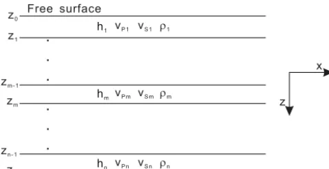
Free surface z0
z1
zm-1
zm
zn-1
zn
x
z h1 vP1 vS1 r1
hm vPm vSm rm
hn vPn vSn rn
Figure 2.1-D layered background model. The thickness, P wave velocity, S wave velocity, and density of each layer are shown.
If we define y1=iuFKH, y2=uFKz, y3=iσHz, and y4=
σzz, Eq. (18) can be changed to the following ordinary
dif-ferential equations:
d
dz
y1
y2
y3
y4
=
0 k 1
µ 0
− λk
λ+2µ 0 0
1
λ+2µ
4k2µ(λ+µ)
λ+2µ −ρω
2 0 0 kλ
λ+2µ
0 −ρω2 −k 0
·
y1
y2
y3
y4
=Fy. (19)
By calculating the eigenvalues and eigenvectors of F, the general solution of Eq. (19) can be written as
y=
1 1 1 1
−i k υS
i k υS
iυP
k −i
υP k iµγ
υS
−iµγ υS
−2iµυP 2iµυP
−2kµ −2kµ −µγ
k −
µγ k
·
e−iυSz 0 0 0
0 eiυSz 0 0
0 0 e−iυPz 0
0 0 0 eiυPz
C1
C2
C3
C4
, (20)
whereC1,C2,C3, andC4correspond to the amplitudes of the upgoing S wave, downgoing S wave, upgoing P wave, downgoing P wave, respectively;p=k
ω,υP =ω
q 1
α2 −p2,
υS=ω
q 1
β2 −p2, andγ=(2k
2−ω2
β2)are the ray
parame-ters. As shown in Fig. 2, the velocities, density, and thick-ness of themth layer are denoted asVP m,VSm,ρm, andhm,
respectively. We define the following matrices for the mth
layer:
Rm=
1 1 1 1
−i k υSm
i k υSm
iυP m
k −i
υP m k iµmγ
υS
−iµmγ υS
−2iµmυP m 2iµmυP m
−2kµm −2kµm − µmγm
k −
µmγm k
,
(21)
H(hm)=
e−iυSz 0 0 0
0 eiυSz 0 0
0 0 e−iυPz 0
0 0 0 eiυPz
. (22)
The relationship between the wave fields atz=zm−1andz=
zmcan be written as
ym−1=RmH(−hm)R−m1ym. (23)
In Eq. (23),Lm=RmH(−hm)R−m1is the propagation
ma-trix. The wave field at the free surface can be represented by
y0=L1· · ·LnRn+1C. (24)
If we consider that the incident plane wave is an upgoing P wave with unit amplitude, then we have
C1=0,
C3= ±isin(θ ). (25)
We define
A=L1· · ·LnRn+1=
a11 a12 a13 a14
a21 a22 a23 a24
a31 a32 a33 a34
a41 a42 a43 a44
. (26)
The values ofy3andy4at the free surface can be written as
y3
y4
z=0
=
a31 a32 a33 a34
a41 a42 a43 a44
0
C2
C3
C4
. (27)
Based on the free surface boundary conditiony3=y4=0, we have
C2
C4
= −C3
a32 a34
a42 a44 −1
a33
a43
. (28)
Substituting Eqs. (25) and (28) into Eq. (23), we obtain the wave field atz=zm. Based on Eq. (23), we can calculate the
3.2 Incident boundary conditions
We assume that the infinite space is composed of the follow-ing hexahedron set:
B=e1, . . ., eN1, eN1+1, . . ., eN1+N2, . . . . (29)
The first N1elements ofB compose the computational do-main (the dodo-main bounded by the blue lines in Fig. 1), and the elements fromN1+1 toN1+N2compose the PML main. We define the set of elements in the computational do-main as
BC=
e1, . . ., eN1 . (30)
A total of N3 elements inBC that contact the boundary of
PML domain are collected in the following set:
BC,B=
n
ej1, . . ., ejN3
o
. (31)
The set of N2 elements that compose the PML domain is given by
BP =
eN1+1, . . ., eN1+N2 . (32)
A total ofN4elements inBP that contact the boundary of the
computational domain are gathered in the following set:
BP ,B=
n
ek1, . . ., ekN4
o
. (33)
We define an operator that maps the elements of vectorAto a target vector At according to the numbering set An. The index number of each elements of setAtin setAis gathered inAn, and we define
hAiA
n =At. (34)
From Eq. (9), we have
¨ UtA
C =
−P
e∈B
Te(M1)−1KeTe(Ut)
AC
=
*
− P
e∈BC∪BP ,B
Te(M1)−1KeTe(Ut) +
AC ,
(35)
whereACis the numbering set of the nodes in the
computa-tional domain. Equation (35) shows that only matrix–vector products in the elements of the computational domain and the elements of the PML domain in contact with the bound-ary of the computational domain contribute to the accelera-tion wave field on the nodes in the computaaccelera-tional domain.
Based on Eq. (35), we have
¨ UtA
C,B =
*
− P
e∈BC∪BP ,B
Te(M)−1KeTe(U
t) +
AC,B
=
*
− P
e∈BC,B∪BP ,B
Te(M)−1KeTe(Ut) +
AC,B
=
*
− P
e∈BC,B
Te(M)−1KeTe(Ut)
+
AC,B
+
*
− P
e∈BP ,B
Te(M)−1KeTe(U
t) +
AC,B ,
(36)
whereAC,B is the numbering set of nodes of the
tional domain located on the interface between the computa-tional and PML domains. The second term of the right side of Eq. (36) can be written as
*
− P
e∈BP ,B
Te(M)−1KeTe(Ut) +
AC,B
=
*
− P
e∈BP ,B
Te(M)−1KeTe U
FK+Us
+
AC,B
=
*
− P
e∈BP ,B
Te(M)−1KeTe(UFK) +
AC,B
+
*
− P
e∈BP ,B
Te(M)−1KeTe(Us)
+
AC,B .
(37)
Equation (37) is the plane-wave incident condition for the computational domain. Based on Eq. (37), we only need to store the boundary wave field *
− P
e∈BP ,B
Te(M)−1KeTe(UFK) +
AC,B
to construct the incident boundary condition for the computational domain. The length of
*
− P
e∈BP ,B
Te(M)−1KeTe(UFK) +
AC,B
is 3 times as long as the number of nodes located on the interface between the computational and PML domains; and it is not necessary to storeUFKon the nodes of the elements inBP ,B.
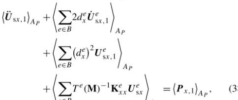
To simplify the discussion, the boundary condition of the first equation of Eq. (16) is discussed. From Eq. (16), we have
¨ Usx,1
AP +
* X
e∈B
2dxeU˙esx,1 +
AP
+
* X
e∈B
dxe2Uesx,1 +
AP
+
* X
e∈B
Te(M)−1KexxUesx +
AP
=Px,1
AP, (38)
whereAP is the numbering set of nodes in the PML domain.
The scattered wave on the interface between the computa-tional domain and the PML domain can be obtained by the following equation:
hUsxiAP ,B= hUtxiAP ,B− hUFKxiAP ,B, (39)
whereAP ,B is the numbering set of the nodes of the PML
domain on the interface.hUsxiAP ,B does not need to be
cal-culated by Eq. (16). From Eqs. (38) and (39), we have
¨ Usx,1
AP−AP ,B +
* P
e∈BP
2dxeU˙e
sx,1+ d
e x
2 Ue
sx,1
+
AP−AP ,B
+
* P
e∈BP
Te(M)−1KeP ,xxUe
sx
+
AP−AP ,B
= hPxiAP−AP ,B.
(40) Considering the other equations of PML ABC, the boundary condition of PML ABC to absorb the scattered waves is
hUsiAP ,B = hUtiAP ,B− hUFKiAP ,B. (41)
In addition to the boundary condition given by Eq. (41), the Dirichlet boundary condition is added to the outer bound-aries of the PML domain, and the natural boundary condi-tion is added to the planes that connect the free surface of the computational domain. Because of the boundary condi-tions, the element-level matrix–vector product is restricted to only the element in the computational domain and the PML domain. Because the boundary conditions in Eqs. (37) and (41) involve the plane-wave fields, we call Eqs. (37) and (41) teleseismic wave incident conditions.
4 Analysis of the computational costs
We use the model in Fig. 1 to quantitatively discuss the com-putational cost of EBE-SEM for teleseismic wave modeling. Because the thickness of the PML domain in our numerical examples is only three elements wide, the number of floating point operations is trivial compared with the computational domain, and the main computational cost of the PML domain
is from the storage requirement of the boundary condition (Eq. 41).
The model is decomposed into 75 000 cubic elements with a size of 2 km×2 km×2 km. The fourth-order interpolation polynomial is used in the space. The time interval is 0.01 s, and the total time for the numerical modeling is 100 s.
The floating point operations in the computational domain are mainly from the element matrix–vector product. A total of 1.0546875×10¹⁰floating point multiplication operations are required in each time step. If a global stiffness matrix is assembled, then the product of the global stiffness matrix and the global solution vector requires a total of 9.35974×10⁹ floating point multiply operations. The computational burden of EBE-SEM is greater than that of the conventional SEM for two reasons: the element stiffness matrix and solution vec-tor product are decomposed into a total of 189 submatrix and solution vector products (Eq. 10), and the acceleration on common nodes shared by the adjacent elements is calcu-lated more than once. However, the number of operations of EBE-SEM increases by only 11.26 %. This increased com-putational amount may be compensated for by the high load balance of EBE-SEM in parallel computing, as will be dis-cussed in the numerical examples.
The memory requirements of EBE-SEM and the conven-tional SEM for teleseismic wave modeling are presented in Table 1. A total of 13.12 GB is required to store the boundary wave field to construct the teleseismic incident conditions. If the classical compressed sparse row (CSR) storage for-mat (Greathouse and Daga, 2014) is used to store the spare stiffness matrix of the conventional SEM, then the storage requirement is 38.76 GB, which is nearly 25 times as large as the storage requirement of EBE-SEM to store the 45 ele-ment submatrices. Two factors contribute to this storage dif-ference. First, CSR must store the row and column informa-tion of the global stiffness matrix in addiinforma-tion to the storage of nonzero elements. Nearly 0.018 and 3.87 GB are required to store the row and column information, respectively. Second, the 45 submatrices for each element are diagonal, i.e., only
(n+1)3nonzero elements of each submatrix must be stored.
5 Numerical examples
Three numerical examples are provided to validate the ef-ficiency of EBE-SEM for teleseismic wave modeling. All three examples use the Gaussian source–time function with a cutoff frequency of 2 Hz (Tong et al., 2014a).
0
20
40
0 20
60
100 40
80 60
0
20
40
60
0
20
40
60
0
20
40
60
0 20
60
100 40
80
0
20
40
60
0
20
40
60
0
20
40
60
0
20
40
60
0 20
60
100 40
80
0 20
60
100 40
80
0 20 40 60 80 100 0 20 40 60 80 100 0 20 40 60 80 100
0 20 40 60 80 100
0 20 40 60 80 100
0 20 40 60 80 100 0 20 40 60 80 100 0 20 40 60 80 100
0 20 40 60 80 100
0 20 40 60 80 100
0 20 40 60 80 100
0 20 40 60 80 100
(a) (b) (c)
(d)
(g)
(j)
(e)
(h)
(k)
(f)
(i)
(l) y(km)
z(km)
x(km) x(km)
z(km)
z(km)
z(km)
y(km)
y(km)
y(km)
y(km)
-0.01 -0.005 0 0.005 0.01
Figure 3.Plane-wave incident on a 1-D crust–upper-mantle model. The snapshots from the top to the bottom are taken att=10, 16, 18, and 22 s, respectively. The left, middle, and right panels are corresponding to snapshots of planes atx=50 km,y=50 km, andz=30 km, respectively. The yellow arrows in(j)and(k)denote the weakly transmitted and reflected S waves. The color scale is shown on the right side of the figure.
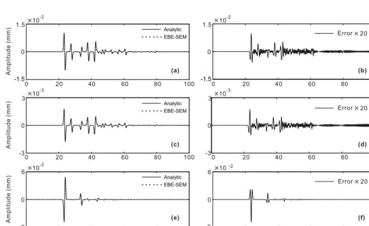
-1.5
Analytic
EBE SEM
-10 1.5
0 -2
0 20 40 60 80 100 -1.50 20 40 60 80 100
1.5
0 10-2
Error 20
(a) (b)
0 20 40 60 80 100
10-3 3
-3 0
3
-3 0
10-3
0 20 40 60 80 100
0 20 40 60 80 100
6
-6 0
6
-6 0
10-2 10-2
0 20 40 60 80 100
Time (s) Time (s)
Amplitude
(mm)
Amplitude
(mm)
Amplitude
(mm)
Analytic
EBE SEM
-Analytic
EBE SEM
-Error 20
Error 20 (c)
(e)
(d)
(f)
Table 1.Memory requirements of EBE-SEM and the conventional SEM for teleseismic wave modeling. All the values are stored in memory with single float precision. GB denotes gigabyte.
Method Stiffness matrix
*
− P
e∈BP ,B
Te(M)−1KeTe(Ut)
+
AC,B
hUFKiAP ,B
EBE-SEM 1.57 GB 6.56 GB 6.56 GB
General SEM 38.76 GB 6.56 GB 6.56 GB
0 2.5 5 7.5
10 10 4
24
2 8 14 20
Figure 5.Parallel efficiency of the EBE-SEM. The red line denotes the theoretical CPU time, and the blue line with circles represents the actual CPU times. The red arrows designate the abnormal CPU times compared with the neighboring CPU times.
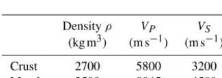
Table 2.Material parameters of the crust–upper-mantle model.
Densityρ VP VS
(kg m3) (m s−1) (m s−1)
Crust 2700 5800 3200
Mantle 3500 8045 4500
located at (60 km, 60 km, 0 km). The computed results are shown in Figs. 3–5.
Figure 3 shows snapshots at four instants. Whent=10 s, the plane wave is still outside the domain (Fig. 3a–c). When
t=16 s, the incident plane wave enters the lower layer of the model (Fig. 3d–f). When t=18 s, the transmitted and reflected P waves are very clear in the plane at y=50 km (Fig. 3h). Figure 3i clearly illustrates that the wavelength in the upper mantle is greater than that in the crust because the velocity of the upper mantle is approximately 1.39 times the velocity of the crust. Whent=22 s, the transmitted P wave is reflected by the free surface, and the Moho-reflected waves are propagating outside the model (Fig. 3k).
To qualitatively evaluate the accuracy of EBE-SEM for teleseismic wave modeling, the synthetic seismology at the station is compared with the reference solution, which is gen-erated by the FK technique. The results are shown in Fig. 4. As depicted in Fig. 4a, the synthetic and reference waveforms show excellent agreement. The direct wave with the largest amplitude is followed by the converted S wave and the crust multiples with relatively small amplitudes. Although the am-plitudes of the crust multiples are small, their phases,
ampli-tudes, and travel times are correctly modeled. The error curve is shown in the right panel of Fig. 4. The maximum relative difference between the numerical solution and the reference solution is less than 5 %, although the numerical method uses only fourth-order interpolation in the space and nearly one spectral-element sampling for the minimal wavelength.
The computation was performed on a workstation with 2 Intel Xeon CPUs (E5-2680 v3) and 128 GB of RAM, and 24 CPU cores were used. The master-slave communication pattern is used in our parallel algorithm, which is similar to that of Komatitsch and Tromp (2002). The parallel effi-ciency is shown in Fig. 5. Because the master–slave commu-nication pattern requires at least two CPU cores to perform the parallel algorithm, the computation time of single CPU core is not shown in Fig. 5. When 2 CPU cores are used, the amount of communication between the CPU cores is negli-gible compared to the amount of computation. If we denote the CPU time when 2 CPU cores are used in parallel compu-tation asT2, the CPU time ofnCPU cores can be estimated byTn=2nT2. The red line in Fig. 5 represents the estimated
CPU times (theoretical times), and the blue line with circles is the practical CPU times. It can be clearly observed that the actual CPU times are extremely close to the theoretical times, even if the number of CPU cores is 24. The red arrows in Fig. 5 indicate the abnormal CPU times. This phenomenon is attributed to the excessive communication amount when the numbers of CPU cores are 18 and 19. However the anomaly is not large compared with the neighboring CPU times. 5.2 Plane-wave incidence to a 3-D model
To demonstrate that EBE-SEM works well in 3-D hetero-geneous models, an abnormal structure with cube shape of an additional 15 % plus wave speeds and density are added at the center of the model in Fig. 1. The size of the abnor-mal structure is 20 km×20 km×20 km. Except for velocity structure, the other computational parameters are the same as those of the first numerical example. The simulation results are shown in Fig. 6.
0
20
40
0 20
60
100 40
80 60
0
20
40
60
0
20
40
60
0
20
40
60
0 20
60
100 40
80
0 20 40 60 80 100 0 20 40 60 80 100 0 20 40 60 80 100
0 20 40 60 80 100 0 20 40 60 80 100 0 20 40 60 80 100
y(km)
z(km)
x(km) x(km)
z(km)
y(km)
y(km)
-0.01 -0.005 0 0.005 0.01
(a) (b) (c)
(d) (e) (f)
Figure 6.Snapshots in a heterogeneous model. The snapshots in the upper and lower panels are taken att=18 and 22 s, respectively. The left, middle, and right panels are snapshots of planes atx=50 km,y=50 km, andz=30 km, respectively. The black arrows in the upper plots indicate the distortion of the wave front because of the velocity anomaly in the media. The yellow arrows in(a)and(b)indicate the scattered waves. The yellow arrows in(d)and(e)denote the scattered waves that are efficiently absorbed by the constructed PML ABC. The color scale is shown on the right side of the figure.
do not reflect back to the interior of the model because of the efficiency of the PML ABC used in this paper.
5.3 Teleseismic waveform misfit gradient
One key advantage of the EBE-SEM is its convenience for constructing the misfit gradient because the element stiffness matrix can easily be assembled based on the tensor product of the submatrices. To illustrate this advantage, we first define the misfit function:
E (m)=1
2 X
s
X
r T
Z
0
[d(t,xr;xs)−s(t,xr;xs)]2dt, (42)
wherem=(lnρ,lnλ,lnµ)represents model parameters,xr
is the station location,xsis the teleseismic incident parame-ters,dis the observed dataset, andsis the synthetic dataset. The cross section between the plane wave and the Moho at
y=0, the incident angle, and the azimuth angle constitute the teleseismic incident parameters. To simplify the discus-sion, this example only considers one source and one station. Based on the continuous adjoint method discussed by Ficht-ner (2011), the adjoint equation is
ρw¨t− ∇ · h
λ (∇ ·wt)I+µ
∇wt+ ∇wTt i
=(d(T−t,xr;xs)−s(T−t,xr;xs)) δ (x−xr) ,
(43) wherewtis the adjoint total wave field. The misfit gradient
∇mEobeys the following equations (Monteiller et al., 2015):
∂E ∂(lnρ)e = −
N T
X
k=0
Wet(T−k1t )MeU¨et(k1t ) 1t
, (44)
∂E ∂(lnλ)e = −
N T
X
k=0
λeWet(T−k1t )KeλUet(k1t ) 1t
, (45)
∂E ∂(lnµ)e = −
N T
X
k=0
2µeWet(T−k1t )KeµUet(k1t ) 1t
,
(46) whereerepresents theeth element; W is the discrete vec-tor ofw;Keλ andKe
µ are the element stiffness matrices for
the misfit gradient calculation, which are presented in Ap-pendix C; andN T is the total time step.KeλandKe
µcan also
be written as a combination of the tensor product of the sub-matrices, which leads to an easy construction of the misfit gradient. The misfit gradients can be written as the gradients with respect to lnρ, lnVP, and lnVS by simple combinations
of Eqs. (44)–(46).
We consider the model in the second numerical example to be the real model and the 1-D layered model in Fig. 1 as the initial model. The observed and synthetic waveforms at the station (red triangle in Fig. 1) are shown in Fig. 7a. As Fig. 7b shows, the time-reversed waveform differences between the observed data and the theoretical data act as the source term in Eq. (43).
Figure 8 shows the constructed misfit gradients in the plane aty=61 km at two time slices. Because of the sin-gularity of the source, large amplitudes are distributed in the vicinity of the adjoint source. The misfit gradient no longer has a banana–doughnut shape (Tromp et al., 2005) but rather is similar to the Greek letter3 (Fig. 8e, f) because of the plane-wave source. The misfit gradient with respect to lnρis much weaker than those for lnVP and lnVS. The extremely
strong negative misfit gradients of lnVP distribute along the
ray path of the directP wave.
6 Discussion and conclusions
ef-1 5.
0
-1 5.
10-2 1.2 10-2
-1.2 0
8
-8 0
8
-4 0
6
-6 0
4
-4 0 10-3
10-2
10-3
10-2
0 20 40 60 80 100 0 20 40 60 80 100
0 20 40 60 80 100 0 20 40 60 80 100
0 20 40 60 80 100
0 20 40 60 80 100
Time (s) Time (s)
Amplitude
(mm)
Amplitude
(mm)
Amplitude
(mm)
(a)
(c)
(e) (f)
(d) (b)
Theoretical data Observed data
Theoretical data Observed data
Theoretical data Observed data
Figure 7.Construction of the adjoint source. In the left panels, the synthetic waveforms from the second example are considered the observed data (blue line), and the synthetic waveforms from the first example are treated as the theoretical data (red line). The rectangular boxes indicate the time window [20, 24] to isolate the waveforms to construct the adjoint source. The top, middle, and bottom panels correspond to thex,y, andzcomponents of the displacement. The three components of the adjoint source–time function is the time-reversed waveform difference between the observed data and the theoretical data.
10 30 50 70 90 10
30
50
10 30 50 70 90 10 30 50 70 90
10 30 50 70 90 10 30 50 70 90
10 30 50 70 90 10
30
50
10
30
50
10
30
50 10
30
50 10
30
50
x (km) x (km) x (km)
z (km)
z (km)
(a) (b) (c)
(f) (e)
(d)
-2E-005 -1E-005 0 1E-005 2E-005
Figure 8.Misfit gradients in the plane aty=61 km at two times. The top and bottom panels correspond tot=18 and 24 s, respectively. The left, middle, and right panels correspond to the misfit gradients in terms ofρ,VP, andVS, respectively. The color scale is shown on the right side of the figure.
ficient method for teleseismic wave forward-modeling and misfit calculation is important. In this work, the EBE-SEM was specially tailored to teleseismic wave modeling and mis-fit gradient calculation. In this approach, the PML ABC is discretized by EBE-SEM, and the method can efficiently ab-sorb scattered teleseismic waves. Teleseismic wave incident conditions are constructed for the computational and PML domains. An economic technique for boundary wave field storage is introduced that can greatly reduce the required amount of computer memory.
The numerical results from the first and second numeri-cal examples demonstrate not only the efficiency of EBE-SEM in modeling teleseismic waves but also the validity of the constructed teleseismic wave incident boundary condi-tion. As shown in the third numerical example, hardly any
extra effort is required to construct the misfit gradient. The EBE-SEM has advantages over the traditional SEM in three respects: the reduction in the required computer memory re-quirement, easy calculation of the misfit gradient, and signif-icant parallelization efficiency.
Appendix A: Element matrices for the computational domain
The element matrices for the computational domain are listed below:
Me=
Me1
Me1 Me
1
, (A1)
Me1=
δij
Z
e
ρφiφjd
, (A2)
Ke=
Ke11 Ke12 Ke13 Ke21 Ke22 Ke23 Ke31 Ke32 Ke33
, (A3)
Ke11=
Z
(λ+2µ)∂φi ∂x
∂φj ∂x +µ
∂φi ∂y ∂φj ∂y + ∂φi ∂z ∂φj ∂z d , (A4)
Ke12=
Z
λ∂φi
∂x ∂φj
∂y +µ ∂φi
∂y ∂φj
∂x d
, (A5)
Ke13=
Z
λ∂φi
∂x ∂φj
∂z +µ ∂φi
∂z ∂φj
∂x d
, (A6)
Ke21=
Z
µ∂φi
∂x ∂φj
∂y +λ ∂φi
∂y ∂φj
∂x d
, (A7)
Ke22=
Z
(λ+2µ)∂φi ∂y
∂φj ∂y +µ
∂φi ∂x ∂φj ∂x + ∂φi ∂y ∂φj ∂y d , (A8)
Ke23=
Z
λ∂φi
∂y ∂φj
∂z +µ ∂φi
∂z ∂φj
∂y d
, (A9)
Ke31=
Z
µ∂φi
∂x ∂φj
∂z +λ ∂φi
∂z ∂φj
∂x d
, (A10)
Ke32=
Z
µ∂φi
∂y ∂φj
∂z +λ ∂φi
∂z ∂φj
∂y d
, (A11)
Ke33=
Z
(λ+2µ)∂φi ∂z
∂φj ∂z +µ
∂φi ∂x ∂φj ∂x + ∂φi ∂y ∂φj ∂y d . (A12)
Appendix B: Element matrices for the PML domain The element matrices for the PML domain are listed below:
Kexx=
Z
e
(λ+2µ)∂φi ∂x
∂φj ∂x d
, (B1)
Keyy=
Z
e µ∂φi
∂y ∂φj
∂y d
, (B2)
Kezz=
Z
e µ∂φi
∂z ∂φj
∂z d
, (B3)
Kexy=
Z
e λ∂φi
∂x ∂φj
∂y d
, (B4)
Keyx=
Z
e µ∂φi
∂y ∂φj
∂x d
, (B5)
Kexz=
Z
e λ∂φi
∂x ∂φj
∂z d
, (B6)
Kezx=
Z
e µ∂φi
∂z ∂φj
∂x d
, (B7)
Kex=
Z
e
(λ+2µ) dx0φi ∂φj
∂x d
, (B8)
Key=
Z
e µdy0φi
∂φj
∂y d, (B9)
Kez=
Z
e µdz0φi
∂φj ∂z d
, (B10)
Dex=
2δij
Z
e
dxeρφiφjd
(B11)
Dey=
2δij
Z
e
dyeρφiφjd
, (B12)
Dez=
2δij
Z
e
dzeρφiφjd
Dexx=
δij
Z
e ρ dxe2
φiφjd
, (B14)
Deyy=
δij
Z
e ρdye
2
φiφjd
, (B15)
Dezz=
δij
Z
e
ρ dze2φiφjd
, (B16)
Dexy=
δij
Z
e
ρdxedyeφiφjd
, (B17)
Dexz=
δij
Z
e
ρdxedzeφiφjd
, (B18)
Dex,y=
δij
Z
e
ρdxe+dyeφiφjd
, (B19)
Dex,z=
δij
Z
e
ρ dxe+dzeφiφjd
. (B20)
wherederepresents the average value of the damping coeffi-cient on the elemente.
Appendix C: Element matrices for the misfit gradient In Eqs. (44) and (45),KeλandKe
µare given by
Keλ=
Keλ11 Keλ12 Keλ13 Keλ21 Keλ22 Keλ23 Keλ31 Keλ32 Keλ33
, (C1)
Keµ=
Keµ
11 0 0
0 Keµ11 0
0 0 Keµ11
, (C2)
Keλ11=
Z
e ∂φi
∂x ∂φj
∂x d
, (C3)
Keλ12=
Z
e ∂φi
∂x ∂φj
∂y d
, (C4)
Keλ13=
Z
e ∂φi
∂x ∂φj
∂z d
, (C5)
Keλ21=
Z
e ∂φi
∂y ∂φj
∂x d
, (C6)
Keλ22=
Z
e ∂φi
∂y ∂φj
∂y d
, (C7)
Keλ23=
Z
e ∂φi
∂y ∂φj
∂z d
, (C8)
Keλ31=
Z
e ∂φi
∂z ∂φj
∂x d
, (C9)
Keλ32=
Z
e ∂φi
∂z ∂φj
∂y d
, (C10)
Keλ33=
Z
e ∂φi
∂z ∂φj
∂z d
, (C11)
Keµ
11=
Z
e
∂φ
i ∂x
∂φj
∂x +
∂φi ∂y
∂φj
∂y +
∂φi ∂z
∂φj ∂z
Competing interests. The authors declare that they have no conflict of interest.
Acknowledgements. We greatly appreciate the detailed suggestions from Michal Afanasiev and the anonymous reviewer. Their valu-able suggestions greatly improved the quality of the paper. This study was supported by the National Natural Science Foundation of China (grant nos. 41230210 and 41604034). Shaolin Liu was financially supported by the China Postdoctoral Science Foundation (grant no. 2015M580085).
Edited by: Michal Malinowski
Reviewed by: Michael Afanasiev and one anonymous referee
References
Capdeville, Y., Chaljub, E., Vilotte, J., and Montagner, J.: Coupling the spectral element method with a modal solution for elastic wave propagation in global Earth models, Geophys. J. Int., 152, 34–67, 2003.
Chen, M., Niu, F., Liu, Q., Tromp, J., and Zheng, X.: Multiparam-eter adjoint tomography of the crust and upper mantle beneath East Asia: 1. Model construction and comparisons, J. Geophys. Res., 120, 22–39, 2015.
Clayton, R. and Engquist, B.: Absorbing boundary condition for acoustic and elastic wave equation, B. Seismol. Soc. Am., 67, 1529–1540, 1977.
Cohen, G.: High-order numerical methods for transient wave equa-tions, Scientific Computation, Springer-Verlag, Berlin Heidel-berg, 2002.
Collino, F. and Tsogka, C.: Application of the perfectly matched absorbing layer model to the linear elastodynamic problem in anisotropic heterogeneous media, Geophysics, 66, 294–307, 2001.
Dablain, M.: The application of high-order differencing to the scalar wave equation, Geophysics, 51, 54–66, 1986.
De Basabe, J. and Sen, M.: Grid dispersion and stability criteria of some common finite-element methods for acoustic and elastic wave equations, Geophysics, 72, T81–T95, 2007.
Fichtner, A.: Full seismic waveform modelling and inversion, Springer-Verlag Berlin Heidelberg, 2011.
Greathouse, J. and Daga, M.: Efficient sparse matrix-vector multi-plication on GPUs using the CSR storage format, International Conference for High Performance Computing, Netwroking, Storage and Analysis, 769–780, 2014.
Haskell, N.: The dispersion of surface waves on multilayered media, B. Seismol. Soc. Am., 43, 17–34, 1953.
Kind, K., Yuan, X., and Kumar, P.: Seismic receiver functions and the lithosphere-astheosphere boundary, Technophysics, 536– 537, 25–43, 2012.
Komatitsch, D. and Tromp, J.: Spectral-element simulations of global seismic wave propagation – I. Validation, Geophys. J. Int., 149, 390–412, 2002.
Komatitsch, D. and Tromp, J.: A perfectly matched layer absorbing boundary condition for the second-order seismic wave equation, Geophys. J. Int., 154, 146–153, 2003.
Komatitsch, D. and Vilotte, J.: The spectral element method: an ef-ficient tool to simulation the seismic response of 2D and 3D ge-ological structures, B. Seismol. Soc. Am., 88, 368–392, 1998. Langston, C.: Corvallis, Oregon, crustal and upper mantel receiver
structure from teleseismic P and S waves, B. Seismol. Soc. Am., 67, 713–724, 1977.
Liu, Q. and Gu, Y.: Seismic imaging: From classical to adjoint to-mography, Tectonophysics, 566–567, 31–66, 2012.
Liu, Q. and Tromp, J.: Finite-frequency kernels based on adjoint method, B. Seismol. Soc. Am., 96, 2383–2397, 2006.
Liu, S., Li, X., Wang, W., and Liu, Y.: A mixed-grid finite element method with PML absorbing boundary conditions for seismic wave modelling, J. Geophys. Eng., 11, 055009, https://doi.org/10.1088/1742-2132/11/5/055009, 2014.
Liu, S., Li, X., Wang, W., and Zhu, T.: Source wavefield recon-struction using a linear combination of the boundary wavefield in reverse time migration, Geophysics, 80, S203–S212, 2015. Liu, S., Yang, D., Lang, C., Wang, W., and Pan, Z.: Modified
symplectic schemes with nearly-analytic discrete operators for acoustic wave simulations, Comp. Phys. Comm., 213, 52–63, 2017a.
Liu, S., Yang, D., and Ma, J.: A modified symplectic PRK scheme for seismic wave modeling, Comp. Geosci., 99, 28–36, 2017b. Monteiller, V., Chevrot, S., Komatitsch, D., and Fuji, N.: A hybrid
method to compute short-period synthetic seismograms of tele-seismic body waves in a 3-D regional model, Geophys. J. Int., 192, 230–247, 2013.
Monteiller, V., Chevrot, S., Komatitsch, D., and Wang, Y.: Three-dimensional full waveform inversion of short-period teleseismic wavefields based upon the SEM-DSM hybrid method, Geophys. J. Int., 202, 811–827, 2015.
Peter, D., Komatitsch, D., Luo, Y., Martin, R., Le Goff, N., Casrotti, E., Le Loher, P., Magnoni, F., Liu, Q., Blitz, C., Nissen-Meyer, T., Basini, P., and Tromp, J.: Forward and adjoint simulations of seismic wave propagation on fully unstructured hexahedral meshes, Geophys. J. Int., 186, 721–739, 2011.
Roecker, S., Baker, D., and McLaughlin, J.: A finite-difference al-gorithm for full waveform teleseismic tomography, Geophys. J. Int., 181, 1017–1040, 2010.
Rondenay, S.: Upper mantle imaging with array recordings of con-verted and scattered teleseismic waves, Surv. Geophys., 30, 377– 405, 2009.
Seriani, G.: A parallel spectral element method for acoustic wave modeling, J. Comp. Acoust., 5, 53–69, 1997.
Seriani, G.: 3-D large-scale wave propagation modelling by spectral element method on Cray T3E multiprocessor, Comput. Method. Appl. M., 164, 235–247, 1998.
Shragge, J., Artman, B., and Wilson, C.: Teleseismic shot-profile migration, Geophysics, 71, S1221–S1229, 2006.
Tape, C., Liu, Q., and Tromp, J.: Finite-frequency tomography using adjoint methods-Methodology and examples using membrance surface waves, Geophys. J. Int., 168, 1105–1129, 2007. Tape, C., Liu, Q., Maggi, A., and Tromp, J.: Adjoint tomography of
the southern California crust, Science, 325, 988–992, 2009. Tong, P., Chen, C., Komatitsch D., Basini, P., and Liu, Q.:
High-resolution seismic array imaging based on an SEM-FK hybrid method, Geophys. J. Int., 197, 369–395, 2014a.
Application to the 1992 Landers earthquake (Mw 7.3) area,
Solid Earth, 5, 1169–1188, https://doi.org/10.5194/se-5-1169-2014, 2014b.
Tong, P., Zhao, D., Yang, D., Yang, X., Chen, J., and Liu, Q.: Wave-equation-based travel-time seismic tomography – Part 1: Method, Solid Earth, 5, 1151–1168, https://doi.org/10.5194/se-5-1151-2014, 2014c.
Tong, P., Komatitsch, D., Tseng, T., Hung, S., Chen, C., Basini, P., and Liu, Q.: A 3-D spectral-element and frequency-wave number hybrid method for high-resolution seismic array imaging, Geo-phys. Res. Lett., 41, 7025–7034, 2015.
Tromp, J., Tape, C., and Liu, Q.: Seismic tomography, adjoint method, time reversal, and banana-doughnut kernels, Geophys. J. Int., 160, 195–216, 2005.
Virieux, J. and Operto, S.: An overview of full-waveform inversion in exploration geophysics, Geophysics, 74, WCC1–WCC26, 2009.
Yang, D., Wang, S., Zhang, Z., and Teng, J.: n-times absorbing boundary conditions for compact finite-difference modeling of acoustic ad elastic wave propagation in 2D TI medium, B. Seis-mol. Soc. Am., 93, 2389–2401, 2003.
Zhang, F., Li, Y., Wu, Q., and Ding, Z.: The P wave velocity struc-ture of upper mantle beneath the North China and surrounding regions from FMTT, Chin. J. Geophys., 54, 1233–1242, 2011 (in Chinese).